Stable Diffusion

Thank you! Your submission has been received!

Oops! Something went wrong while submitting the form.

Results

Sort By:

Title

Date

Dynamic shapes support in OpenVINO JIT compiler boosts inference performance by 40%

April 28, 2025

Authors: Ivan Novoselov, Alexandra Sidorova, Vladislav Golubev, Dmitry Gorokhov

Introduction

Deep learning (DL) has become a powerful tool for addressing challenges in various domains like computer vision, generative AI, and natural language processing. Industrial applications of deep learning often require performing inference in resource-constrained environments or in real time. That’s why it’s essential to optimize inference of DL models for particular use cases, such as low-latency, high-throughput or low-memory environments. Thankfully, there are several frameworks designed to make this easier, and OpenVINO stands out as a powerful tool for achieving these goals.

OpenVINO is an open-source toolkit for optimization and deployment of DL models. It demonstrates top-tier performance across a variety of hardware including CPU (x64, ARM), AI accelerators (Intel NPU) and Intel GPUs. OpenVINO supports models from popular AI frameworks and delivers out-of-the box performance improvements for diverse applications (you are welcome to explore demo notebooks). With ongoing development and a rapidly growing community, OpenVINO continues to evolve as a versatile solution for high-performance AI deployments.

The primary objective of OpenVINO is to maximize performance for a given DL model. To do that, OpenVINO applies a set of hardware-dependent optimizations The optimizations are typically performed by replacing a target group of operations with a custom operation that can be executed more efficiently. In the standard approach, these custom operations are executed using handcrafted implementations. This approach is highly effective when optimizing a few patterns of operations. On the other hand, it lacks scalability and thus requires too much effort when dozens of similar patterns should be supported.

To address this limitation and build a more flexible optimization engine, OpenVINO introduced Snippets, an integrated Just-In-Time (JIT) compiler for computational graphs. Snippets provide a flexible and scalable approach for operation fusions and enablement. The graph compiler automatically identifies subgraphs of operations that can benefit from fusion and combines them into a single node, referred to as “Subgraph”. Snippets then apply a series of optimizing transformations to the subgraph and JIT compile an executable that efficiently performs the computations defined by the subgraph.

One of the most common examples of such subgraphs is Scaled Dot-Product Attention (SDPA) pattern. SDPA it is a cornerstone of transformer-based architectures which dominate most of the state-of-the-art models. There are numerous SDPA pattern flavours and variations dictated by model-specific adjustments or optimizations. Thanks to compiler-based design, Snippets support most of these configurations. Fig. 1 illustrates the general structure of the SDPA pattern supported by Snippets, highlighting its adaptability to different model requirements:

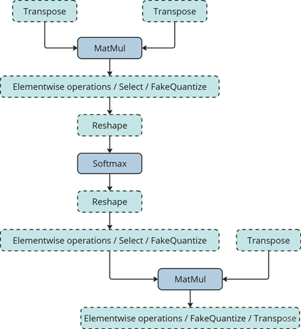
Figure 1. SPDA variations supported by Snippets. Blocks with a dashed border denote optional operations. The operations listed inside the block can be in any order. The semantics of the operations are described in the *OpenVINO documentation*.

Note that SDPA has quadratic time and memory complexity with respect to sequence length. It means that by fusing SDPA-like patterns, Snippets significantly reduce memory consumption and accelerate transformer models, especially for large sequence lengths.

Snippets effectively optimized SDPA patterns but had a key limitation: they did not support dynamic shapes. In other words, input shapes must be known at the model compilation stage and can’t be changed in runtime. This limitation reduced the applicability of Snippets to many real-world scenarios where input shapes are not known in advance. While it is technically possible to JIT-compile a new binary for each unique set of input shapes, this approach introduces significant recompilation overheads, often negating the performance gains from SDPA fusion.

Fortunately, this static-shape limitation is not inherent to Snippets design. They can be modified to support dynamic shapes internally and generate shape-agnostic binaries. In this post, we discuss Snippets architecture and the challenges we faced during this dynamism enablement.

Architecture

The first step of the Snippets pipeline is called Tokenization. It is applied to an ov::Model, which represents OpenVINO Intermediate Representation (IR). It’s a standard IR in the OV Runtime you can read more about it here or here. The purpose of this stage is to identify parts of the initial model that can be lowered by Snippets efficiently. We are not going to discuss Tokenization in detail because this article is mostly focused on the dynamism implementation. A more in-depth description of the Tokenization process can be found in the Snippets design guide. The key takeaway for us here is that the subsequent lowering is performed on a part of the initial ov::Model. We will call this part Subgraph, and the Subgraph at first is also represented as an ov::Model.

Now let’s have a look at the lowering pipeline, its schematic representation is shown on Fig.2a. As can be seen from the picture, the lowering process consists of three main phases: Data Flow Optimizations, Control Flow Optimizations and Binary Code Generation. Let’s briefly discuss each of them.

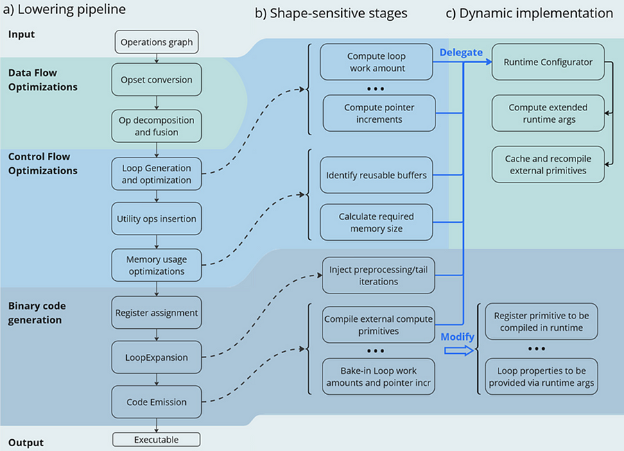
Lowering Pipeline

The first stage is the Data Flow optimizations. As we mentioned above, this stage’s input is a part of the initial model represented as an ov::Model. This representation is very convenient for high-level transformations such as opset conversion, operations’ fusion/decomposition and precision propagation. Here are some examples of the transformations performed on this stage:

ConvertPowerToPowerStatic — operation Power with scalar exponent input is converted to PowerStatic operation from the Snippets opset. The PowerStatic ops then use the values of the exponents to produce more optimal code.
FuseTransposeBrgemm — Transpose operations that can be executed in-place with Brgemm blocks are fused into the Brgemm operations.
PrecisionPropagation pass automatically inserts Converts operations between the operations that don’t natively support the desired execution precision.

The next stage of the lowering process is Control Flow optimizations (or simply CFOs). Note that the ov::Model is designed to primarily describe data flow, so is not very convenient for CFOs. Therefore, we had to develop our own IR (called Linear IR or simply LIR) that explicitly represents both control and data flows, you can read more about LIR here. So the ov::Model IR is converted to LIR before the start of the CFOs.

As you can see from the Fig.2a, the Control Flow optimization pipeline could roughly be divided into three main blocks. The first one is called Loop Generation and Optimization. This block includes all loop-related optimizations such as automatic generation of loops based on the input tensors’ dimensions, loop fusion and blocking loops generation.

The second block of Control Flow optimizations is called Utility Ops Insertion. We need this block of transformations here to insert utility operations that depend on loop control structures, specifically on their entry and exit points locations. For example, operations like Load, Store, MemoryBuffer, LoopBegin and LoopEnd are inserted during this stage.

The last step of CFO is the Memory Usage Optimizations block. These transformations determine required sizes of internal memory buffers, and analyze how much of that memory can be reused. A graph coloring algorithm is employed to minimize memory consumption.

Now all Control Flow optimizations are performed, and we are ready to proceed to the next stage of the lowering pipeline — Binary Code Generation (BCG). As one can see from Fig.2a, this stage consists of three substages. The first one is Register Assignment. We use a fairly standard approach here: calculate live intervals first and use the linear scan algorithm to assign abstract registers that are later mapped to physical ones.

The next BSG substage is Loop Expansion. To better understand its purpose, let’s switch gears for a second and think about loops in general. Sometimes it’s necessary to process the first or the last iteration of a loop in a special way. For example, to initialize a variable or to process blocking loops’ tails. The Loop Expansion pass unrolls these special iterations (usually the first or the last one) and explicitly injects them into the IR. This is needed to facilitate subsequent code emission.

The final step of the BCG stage is Code Emission. At this stage, every operation in our IR is mapped to a binary code emitter, which is then used to produce a piece of executable code. As a result, we produce an executable that performs calculations described by the initial input ov::Model.

Dynamic Shapes Support

Note that some stages of the lowering pipeline are inherently shape-sensitive, i.e. they rely on specific values of input shapes to perform optimizations. These stages are schematically depicted on the Fig. 2b.

As can be seen from the picture, shapes are used to determine loops’ work amounts and pointer increments that should be performed on every iteration. These parameters are later baked into the executable during Code Emission. Another example is Memory Usage Optimizations, since input shapes are needed to calculate memory consumption. Loop Expansion also relies on input shapes, since it needs to understand if tail processing is required for a particular loop. Note also that Snippets use compute primitives from third-party libraries, BRGEMM block from OneDNN for example. These primitives should as well be compiled with appropriate parameters that are also shape-sensitive.

One way to address these challenges is to rerun the lowering pipeline for every new set of input shapes, and to employ caching to avoid processing the same shapes twice. However, preliminary analysis indicated that this approach is too slow. Since this re-lowering needs to be performed in runtime, the performance benefit provided by Snippets is essentially eliminated by the recompilation overheads.

The performed experiments thus indicate that we can afford to run the whole lowering pipeline only once during the model compilation stage. Only some minor adjustments can be made at runtime. In other words, we need to remove all shape-sensitive logic from the lowering pipeline and perform the compilation without it. The remaining shape-sensitive transformations should be performed at runtime. Of course, we would also need to share this runtime context with the compiled shape-agnostic kernel. The idea behind this approach is schematically represented on Fig. 2c.

As one can see from the picture, all the shape-sensitive transformations are now performed by a new entity called Runtime Configurator. It’s probably easier to understand its purpose in some examples.

Imagine that we need to perform a unary operation get_result(X) on an input tensor X — for example, apply an activation function. To do this, we need to load some input data from memory into registers, perform the necessary computations and write the results back to memory. Of course this read-compute-write sequence should be done in a loop since we need to process the entire input tensor. These steps are described in more detail in Fig. 3 using pseudocode. Fig. 3a corresponds to a static kernel while Fig. 3b represents a dynamic one.

Let’s consider the static kernel as a starting point. As the first step, we need to load pointers to input and output memory blobs to general-purpose registers (or simply GPRs) denoted G_IN and G_OUT on the picture. Then we initialize another GPR that stores the loop work amount (G_WA). Note that the loop is used to traverse the input tensor, so the loop’s work amount is fixed because the tensor’s dimensions are also known at the BCG stage. The next six steps in the picture (3 to 8) are in the loop’s body.

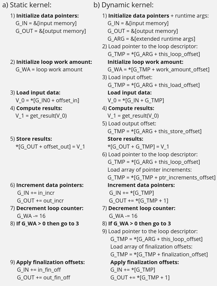
Figure 3. Pseudocode for performing an unary operation “get_result” for a) — static and b) — dynamic kernels. Note that general-purpose and vector registers are denoted with “G_” and “V_” prefixes, respectively.

In step 3, we load input data into a vector register V_0, note that the appropriate pointer is already loaded to G_IN, and offset_in is fixed because the input tensor is static. Next, we apply our get_result function to the data in V_0 and place the result in a spare vector register V_1. Now we need to store V_1 back to memory, which is done on step 5. Note that offset_out is also known in the static case. This brings us almost to the end of the loop’s body, and the last few things we need to do are to increment data pointers (step 6), decrement loop counter (step 7), and jump to the beginning of the body, if needed (step 8).

Finally, we need to reset data pointers to their initial values after the loop is finished, which is done using finalization offsets on step 9. Note that this step could be omitted in our simplified example, but it’s often needed for more complicated use cases, such as when the data pointers are used by subsequent loops.

Now that we understand the static kernel, let’s consider the dynamic one, which is shown in Fig. 3b. Unsurprisingly, the dynamic kernel performs essentially the same steps as the static one, but with additional overhead due to loading shape-dependent parameters from the extended runtime arguments. Take step 1 as an example, we need to load not only memory pointers (to G_IN and G_OUT), but also a pointer to the runtime arguments prepared by the runtime configurator (to G_ARG).

Next, we need to load a pointer to the appropriate loop descriptor (a structure that stores loops’ parameters) to a temporary register G_TMP, and only then we can initialize the loop’s work amount register G_WA (step 2). Similarly, in order to load data to V_0, we need to load a runtime-calculated offset from the runtime arguments in step 3. The computations in step 4 are the same as in the static case, since they don’t depend on the input shapes. Storing the results to memory (step 5) requires reading a dynamic offset from the runtime arguments again. Next, we need to shift the data pointers, and again we have to load the increments from the corresponding loop descriptor in G_ARG because they are also shape-dependent, as the input tensor can be strided. The following two steps 7 and 8 are the same as in the static case, but the finalization offsets are also dynamic, so we have to load them from G_ARG yet again.

As one can see from Fig. 3, dynamic kernels incorporate additional overhead due to reading the extended runtime parameters provided by the runtime configurator. However, this overhead could be acceptable as long as the input tensor is large enough (Load/Store operations would take much longer than reading runtime arguments from L1) and the amount of computation is sufficient (get_results is much larger than the overhead). Let’s consider the performance of this design in the Results section to see if these conditions are met in practical use cases.

Results

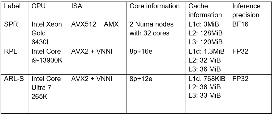
We selected three platforms to evaluate the dynamic pipeline’s performance in Snippets. These platforms represent different market segments: the Intel Core machine is designed for high-performance user and professional tasks. While the Intel Xeon is a good example of enterprise-level hardware often used in data centers and cloud computing applications. The information about the platforms is described in the table below:

As discussed in the Introduction, Snippets support various SDPA-like patterns which form the backbone of Transformer models. These models often work with input data of arbitrary size (for example, sequence length in NLP). Thus, dynamic shapes support in Snippets can efficiently accelerate many models based on Transformer architecture with dynamic inputs.

We selected 43 different Transformer-models from HuggingFace to measure how the enablement of dynamic pipeline in Snippets affects performance. The models were downloaded and converted to OpenVINO IRs using Optimum Intel. These models represent different domains and were designed to solve various tasks in natural language processing, text-to-image image generation and speech recognition (see full model list at the end of the article). What unifies all these models is that they all contain SDPA subgraph and thus can be accelerated by Snippets.

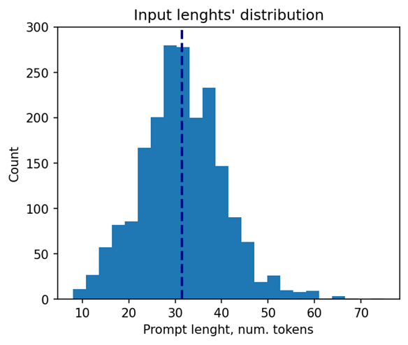
Let’s take a closer look at the selected models. The 37 models of them solve different tasks in natural language processing. Their performance was evaluated using a list of 2000 text sequences with different lengths, which also mimics the real-word scenario. The total processing time of all the sequences were measured in every experiment. Note that the text sequences were converted to model inputs using model-specific tokenizers prior to the benchmarking. The lengths’ distribution of the tokenized sequences is shown on Fig. 4. As can be seen from the picture, the distribution is close to normal with the mean length of 31 tokens.

*Figure 4. Distribution of input prompt lengths that were used for benchmarking of NLP models. Vertical dashed line denotes the mean of the distribution.*

The other 6 models of the selected model scope solve tasks in text-to-image image generation (Stable Diffusion) and speech recognition (Whisper). These models decompose into several smaller models after export to OpenVINO representation using Optimum Intel. Stable Diffusion topology is decomposed into Encoder, Diffuser and Decoder. The most interesting model here is Diffuser because it’s the one responsible for denoising of the latent image representation. This generation stage is repeated several times, so it is the most computationally intensive, which mostly effects on the generation time of the image. Whisper is also decomposed into Encoder and Decoder, which also contain SDPA patterns. The Encoder encodes the spectrogram from the feature extractor to form a sequence of encoder hidden states. Then, the decoder autoregressively predicts text tokens, conditional on both the previous tokens and the encoder hidden states. Currently, Snippets support efficient execution of SDPA only in Whisper Encoder, while Decoder is a subject for future support. To evaluate the inference performance of Stable Diffusion and Whisper models, we collect generation time of image/speech using LLM Benchmark from openvino.genai. This script provides a unified approach to estimate performance for GenAI workloads in OpenVINO.

Performance Improvements

Note that the main goal of these experiments is to estimate the impact of Snippets on the performance of the dynamic pipeline. To do that, we performed two series of experiments for every model. The first version of experiments is with disabled Snippets tokenization. In this case, all operations from the SDPA pattern are performed on the CPU plugin side as stand-alone operations. The second variant of experiments — with enabled Snippets tokenization. The relative difference between numbers collected on these two series of experiments is our performance metric — speedup, the higher the better. Firstly, let’s take a closer look at the resulting speedups for the BERT models which are depicted on Fig. 5.

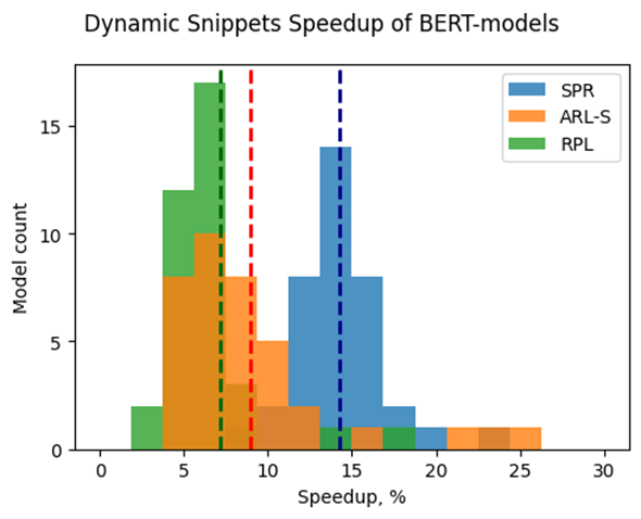
*Figure 5. Impact of Snippets enablement on the performance of BERT-models. Vertical dashed lines denote mean values similar to Fig.4.*

The speedups on RPL range from 3 to 18%, while on average the models are accelerated by 7%. The ARL-S speedups are somewhat higher and reach 20–25% for some models, the average acceleration factor is around 9%. The most affected platform is SPR, it has the highest average speedup of 15 %.

One can easily see from these numbers that both average and maximum speedups depend on the platform. To understand the reason for this variation, we should recall that the main optimizations delivered by Snippets are vertical fusion and tiling. These optimizations improve cache locality and reduce the memory access overheads. Note SPR has the largest caches among the examined platforms. It also uses BF16 precision that takes two times less space per data element compared to F32 used on ARL-S and RPL. Finally, SPR has AMX ISA extension that allows it to perform matrix multiplications much faster. As a result, SDPA execution was more memory bound on SPR, so this platform benefited the most from the Snippets enablement. At the same time, the model speedups on ARL-S and RPL are almost on the same level. These platforms use FP32 inference precision while SPR uses BF16, and they have less cache size than SPR.

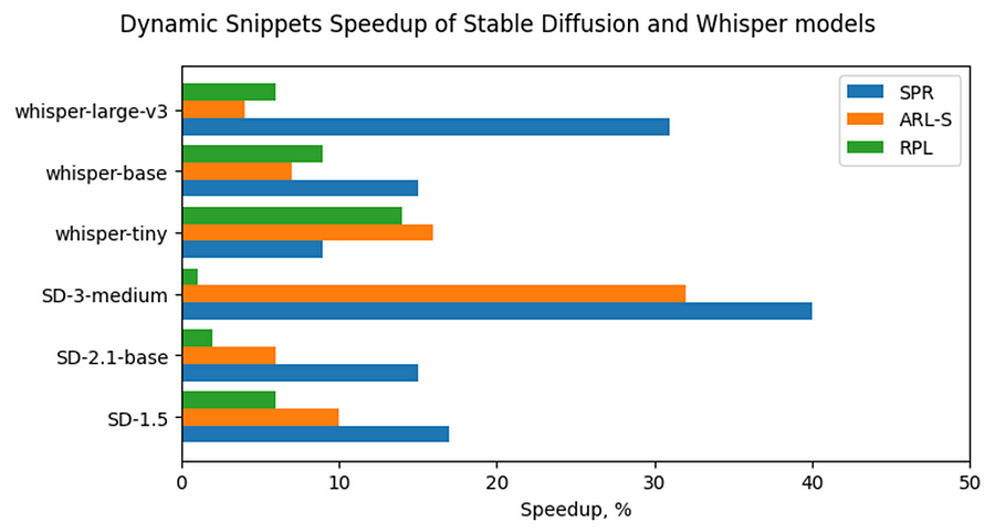
*Figure 6. Impact of Snippets enablement on the performance of Stable Diffusion and Whisper models*

Now, let’s consider Stable Diffusion and Whisper topologies and compare their speedups with some of BERT-like models. As can be seen from the Fig. 6, the most accelerated Stable Diffusion topology is StableDiffusion-3-medium — almost 33% on ARL-S and 40% on SPR. The most accelerated model in this Stable Diffusion pipeline is Diffuser. This model has made a great contribution to speeding up the entire image generation time. The reason the Diffuser benefits more from Snippets enablement is that they use larger sequence lengths and embedding sizes. It means that their attention blocks process more data and are more memory constrained compared to BERT-like models. As a result, the Diffuser models in Stable Diffusion benefit more from the increased cache locality provided by Snippets. This effect is more pronounced on the SPR than on the ARL-S and RPL for the reasons discussed above (cache sizes, BF16, AMX).

The second most accelerated model is whisper-large-v3–30% on SPR. This model has more parameters than base and tiny models and process more Mel spectrogram frequency bins than they. It means that Encoder of whisper-large-v3 attention blocks processes more data, like Diffuser part of Stable Diffusion topologies. By the same reasons, whisper-large-v3 benefits more (increased cache locality provided by Snippets).

Memory Consumption Improvements

Another important improvement from Snippets using is reduction of memory consumption. Snippets use vertical fusion and various optimizations from Memory Usage Optimizations block (see the paragraph “Lowering Pipeline” in “Architecture” above for more details). Due to this fact, Subgraphs tokenized by Snippets consumes less memory than the same operations performed as stand-alone in CPU Plugin.

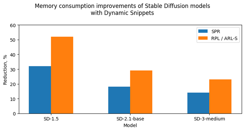
*Figure 7. Impact of Snippets enablement on the memory consumption of image generation using Stable Diffusion models.*

Let’s take a look at the Fig. 7 where we can see improvements in image generation memory consumption using Stable Diffusion pipelines from Snippets usage. As discussed above, the attention blocks in the Diffuser models from these pipelines process more data and consume more memory. Because of that, the greatest impact on memory consumption from using Snippets is seen on Stable Diffusion pipelines. For example, memory consumption of image generation is reduced by 25–50% on RPL and ARL-S platforms with FP32 inference precision and by 15–30% on SPR with BF16 inference precision.

Thus, one of the major improvements from using Snippets is memory consumption reduction. It allows extending the range of platforms which are capable to infer such memory-intensive models as Stable Diffusion.

Conclusion

Snippets is a JIT compiler used by OpenVINO to optimize performance-critical subgraphs. We briefly discussed Snippets’ lowering pipeline and the modifications made to enable dynamism support. After these changes, Snippets generate shape-agnostic kernels that can be used for various input shapes without recompilation.

This design was tested on realistic use cases across several platforms. As a result, we demonstrate that Snippets can accelerate BERT-like models by up to 25%, Stable Diffusion and Whisper pipelines up to 40%. Additionally, Snippets can significantly reduce memory consumption by several tens of percent. Notably, these improvements result from more optimal hardware utilization, so the models’ accuracy remains unaffected.

References

Model list can be found here: https://gist.github.com/a-sidorova/2c2aa584922389138e5ccbad0e0c773b

Intel Xeon Gold 6430L: https://www.intel.com/content/www/us/en/products/sku/231737/intel-xeon-gold-6430-processor-60m-cache-2-10-ghz/specifications.html

Intel Core i9-13900K: https://www.intel.com/content/www/us/en/products/sku/230496/intel-core-i913900k-processor-36m-cache-up-to-5-80-ghz/specifications.html

Intel Core Ultra 7 265K: https://www.intel.com/content/www/us/en/products/sku/241063/intel-core-ultra-7-processor-265k-30m-cache-up-to-5-50-ghz/specifications.html

Notices & Disclaimers

Performance varies by use, configuration, and other factors. Learn more on the Performance Index site.

No product or component can be absolutely secure. Your costs and results may vary. Intel technologies may require enabled hardware, software or service activation.

‍

OpenVINO Latent Consistency Model C++ pipeline with LoRA model support

January 25, 2024

Introduction

Latent Consistency Models (LCMs) is the next generation of generative models after Latent Diffusion Models (LDMs). While Latent Diffusion Models (LDMs) like Stable Diffusion are capable of achieving the outstanding quality of generation, they often suffer from the slowness of the iterative image denoising process. LCM is an optimized version of LDM. Inspired by Consistency Models (CM), Latent Consistency Models (LCMs) enabled swift inference with minimal steps on any pre-trained LDMs, including Stable Diffusion. The Consistency Models is a new family of generative models that enables one-step or few-step generation. More details about the proposed approach and models can be found using the following resources: project page, paper, original repository.

This article will demonstrate a C++ application of the LCM model with Intel’s OpenVINO™ C++ API on Linux systems. For model inference performance and accuracy, the C++ pipeline is well aligned with the Python implementation.

The full implementation of the LCM C++ demo described in this post is available on the GitHub: openvino.genai/lcm_dreamshaper_v7.

Model Conversion

To leverage efficient inference with OpenVINO™ runtime on Intel platforms, the original model should be converted to OpenVINO™ Intermediate Representation (IR).

LCM model

Optimum Intel can be used to load SimianLuo/LCM_Dreamshaper_v7 model from Hugging Face Hub and convert PyTorch checkpoint to the OpenVINO™ IR on-the-fly, by setting export=True when loading the model, like:

from optimum.intel.openvino import OVLatentConsistencyModelPipeline

model = OVLatentConsistencyModelPipeline.from_pretrained("SimianLuo/LCM_Dreamshaper_v7", export=True)
model.save_pretrained("ov_lcm_model")

Tokenizer

OpenVINO Tokenizers is an extension that adds text processing operations to OpenVINO Inference Engine. In addition, the OpenVINO Tokenizers project has a tool to convert a HuggingFace tokenizer into OpenVINO IR model tokenizer and detokenizer: it provides the convert_tokenizer function that accepts a tokenizer Python object and returns an OpenVINO Model object:

from transformers import AutoTokenizer
from openvino_tokenizers import convert_tokenizer
from openvino import compile_model, save_model

hf_tokenizer = AutoTokenizer.from_pretrained(tokenizer_path)
ov_tokenizer_encoder = convert_tokenizer(hf_tokenizer)
save_model(ov_tokenizer_encoder, "ov_tokenizer.xml")

Note: Currently OpenVINO Tokenizers can be inferred on CPU devices only.

Conversion step

You can find the full script for model conversion at the original repo.

Note: The tutorial assumes that the current working directory is and <openvino.genai repo>/image_generation/lcm_ dreamshaper_v7/cpp all paths are relative to this folder.

Let’s prepare a Python environment and install dependencies:

conda create -n openvino_lcm_cpp python==3.10
conda activate openvino_lcm_cpp
conda install -c conda-forge 'openvino>=2023.3.0'
python -m pip install -r scripts/requirements.txt
python -m pip install ../../../thirdparty/openvino_contrib/modules/custom_operations/[transformers]

Now we can use the script scripts/convert_model.py to download and convert models:

cd scripts
python convert_model.py -lcm "SimianLuo/LCM_Dreamshaper_v7" -t FP16

C++ Pipeline

Pipeline flow

Let’s now talk about the logical structure of the LCM model pipeline.

Just like the classic Stable Diffusion pipeline, the LCM pipeline consists of three important parts:
- A text encoder to create a condition to generate an image from a text prompt.
- U-Net for step-by-step denoising the latent image representation.
- Autoencoder (VAE) for decoding the latent space to an image.

The pipeline takes a latent image representation and a text prompt transformed to text embedding via CLIP’s text encoder as an input. The initial latent image representation is generated using random noise generator. LCM uses a guidance scale for getting time step conditional embeddings as input for the diffusion process, while in Stable Diffusion, it used for scaling output latents.

Next, the U-Net iteratively denoises the random latent image representations while being conditioned on the text embeddings. The output of the U-Net, being the noise residual, is used to compute a denoised latent image representation via a scheduler algorithm. LCM introduces its own scheduling algorithm that extends the denoising procedure introduced by denoising diffusion probabilistic models (DDPMs) with non-Markovian guidance. The denoising process is repeated for a given number of times to step-by-step retrieve better latent image representations. When complete, the latent image representation is decoded by the decoder part of the variational auto encoder.

The C++ implementations of the scheduler algorithm and LCM pipeline are available at the following links: LCM Scheduler, LCM Pipeline.

LoRA support

LoRA (Low-Rank Adaptation) is a training technique for fine-tuning Stable Diffusion models. There are various LoRA models available on https://civitai.com/tag/lora.

The main idea for LoRA weights enabling, is to append weights onto the OpenVINO LCM models at runtime before compiling the Unet/text_encoder model. The method is to extract LoRA weights from safetensors file, find the corresponding weights in Unet/text_encoder model and insert the LoRA bias weights. The common approach to add LoRA weights looks like:

The original LoRA safetensor model is loaded via safetensors.h. The layer name and weight of LoRA are modified with Eigen Lib and inserted into Unet/text_encoder OpenVINO model using ov::pass::MatcherPass - you can see the implementation in the file common/diffusers/src/lora.cpp.

To run the LCM demo with the LoRA model, first download LoRA, for example: LoRa/Soulcard.

Build and Run LCM demo

Let’s start with the dependencies installation:‍

conda activate openvino_lcm_cpp
conda install -c conda-forge eigen c-compiler cxx-compiler make

Now we can build the application:

cmake -DCMAKE_BUILD_TYPE=Release -S . -B build
cmake --build build --config Release --parallel
cd build

‍‍And finally we’re ready to run the LCM demo. By default the positive prompt is set to: “a beautiful pink unicorn”.

Please note, that the quality of the resulting image depends on the quality of the random noise generator, so there is a difference for output images generated by the C++ noise generator and the PyTorch generator. Use oprion -r to read the PyTorch generated noise from the provided textfiles for the alignment with Python pipeline.
‍

Note: Run ./lcm_dreamshaper -h to see all the available demo options

Let’s try to run the application in a few modes:

Read the numpy latent input and noise for scheduler instead of C++ std lib for the alignment with Python pipeline: ./lcm_dreamshaper -r‍

Generate image with C++ std lib generated latent and noise : ./lcm_dreamshaper

‍

‍

Generate image with Soulcard LoRa and C++ generated latent and noise: ./lcm_dreamshaper -r -l path/to/soulcard.safetensors

‍

Introduction

Stable Diffusion (SD) is a state-of-the-art latent text-to-image diffusion model that generates photorealistic images from text. Recently, many fine-tuning technologies proposed to create custom Stable Diffusion pipelines for personalized image generation, such as Textual Inversion, Low-Rank Adaptation (LoRA). We’ve already published a blog for enabling LoRA with Stable Diffusion + ControlNet pipeline.

In this blog, we will focus on enabling pre-trained textual inversion with Stable Diffusion via Optimum-Intel. The feature is available in the latest Optimum-Intel, and documentation is available here.

Textual Inversion is a technique for capturing novel concepts from a small number of example images in a way that can later be used to control text-to-image pipelines. It does so by learning new “words” in the embedding space of the pipeline’s text encoder.

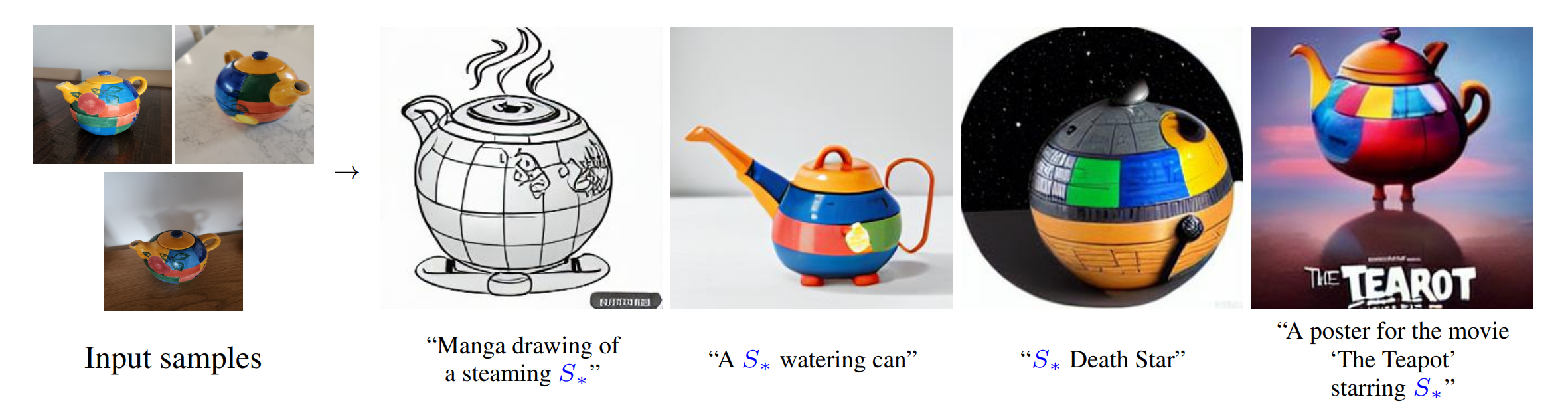
Figure1. Textual Inversion sample: injecting user-specific concepts into new scenes

As Figure 1 shows, you can teach new concepts to a model such as Stable Diffusion for personalized image generation using just 3-5 images.

Hugging Face Diffusers and Stable Diffusion Web UI provides useful tools and guides to train and save custom textual inversion embeddings. The pre-trained textual inversion embeddings are widely available in sd-concepts-library and civitai, which can be loaded for inference with the StableDiffusionPipeline using Pytorch as the runtime backend.

Here is an example to load pre-trained textual inversion embedding sd-concepts-library/cat-toy to inference with Pytorch backend.

from diffusers import StableDiffusionPipeline

model_id = "runwayml/stable-diffusion-v1-5"
pipe = StableDiffusionPipeline.from_pretrained(model_id)
pipe.load_textual_inversion("sd-concepts-library/cat-toy")
prompt = "A <cat-toy> backpack"

image = pipe(prompt, num_inference_steps=50).images[0]
image.save("cat-backpack.png")

Optimum-Intel provides the interface between the Hugging Face Transformers and Diffusers libraries to leverage OpenVINO^TMruntime to accelerate end-to-end pipelines on Intel architectures.

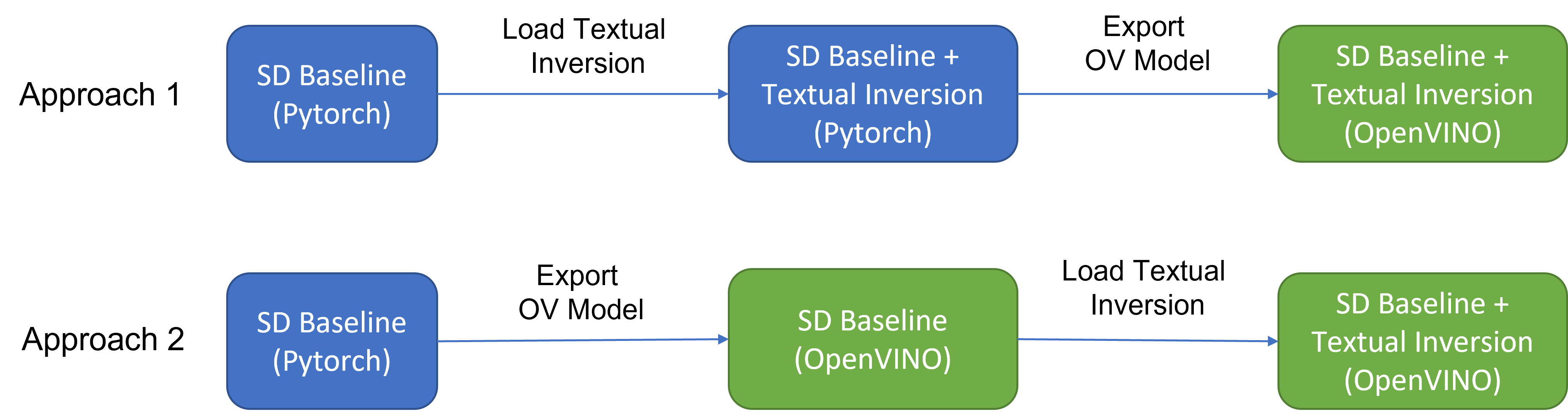
Figure2: Two approaches to enable textual inversion with Stable Diffusion

As Figure 2 shows that two approaches are available to enable textual inversion with Stable Diffusion via Optimum-Intel.

Although approach 1 seems quite straightforward and does not need any code modification in Optimum-Intel, the method requires the re-export ONNX model and then model conversion to the OpenVINO^TM IR model whenever the SD baseline model is merged with anew textual inversion.

Instead, we propose approach 2 to support OVStableDiffusionPipelineBase to load pre-trained textual inversion embeddings in runtime to save disk storage while keeping flexibility.

Save disk storage: We only need to save an SD baseline model converted to OpenVINO^TM IR (e.g.: SD-1.5 ~5GB) and multiple textual embeddings (~10KB-100KB), instead of multiple SD OpenVINO^TM IR with textual inversion embeddings merged (~n *5GB), since disk storage is limited, especially for edge/client use case.
Flexibility: We can load (multiple) pre-trained textual inversion embeddings in the SD baseline model in runtime quickly, which supports the combination of embeddings and avoid messing up the baseline model.

‍

How to enable textual inversion in runtime?

We implemented OVTextualInversionLoaderMixinbased on diffusers.loaders.TextualInversionLoaderMixin with the following features:

Load and parse textual embeddings saved as*.bin, *.pt, *.safetensors as a list of Tensors.
Update tokenizer for new “words” using new token id and expand vocabulary size.
Update text encoder embeddings via InsertTextEmbedding class based on OpenVINO^TMngraph transformation.

‍

For the implementation details of OVTextualInversionLoaderMixin, please refer to here.

Here is the sample code for InsertTextEmbedding class:

class InsertTextEmbedding(MatcherPass):
    r"""
    OpenVINO ngraph transformation for inserting pre-trained texual inversion embedding to text encoder
    """

    def __init__(self, token_ids_and_embeddings):
        MatcherPass.__init__(self)
        self.model_changed = False
        param = WrapType("opset1.Constant")

        def callback(matcher: Matcher) -> bool:
            root = matcher.get_match_root()
            if root.get_friendly_name() == TEXTUAL_INVERSION_EMBEDDING_KEY:
                add_ti = root
                consumers = matcher.get_match_value().get_target_inputs()
                for token_id, embedding in token_ids_and_embeddings:
                    ti_weights = ops.constant(embedding, Type.f32, name=str(token_id))
                    ti_weights_unsqueeze = ops.unsqueeze(ti_weights, axes=0)
                    add_ti = ops.concat(
                        nodes=[add_ti, ti_weights_unsqueeze],
                        axis=0,
                        name=f"{TEXTUAL_INVERSION_EMBEDDING_KEY}.textual_inversion_{token_id}",
                    )

                for consumer in consumers:
                    consumer.replace_source_output(add_ti.output(0))

                # Use new operation for additional matching
                self.register_new_node(add_ti)

            # Root node wasn't replaced or changed
            return False

        self.register_matcher(Matcher(param, "InsertTextEmbedding"), callback)

InsertTextEmbeddingclass utilizes OpenVINO^TM ngraph MatcherPass function to insert subgraph into the model. Please note, the MacherPass function can only filter layers by type, so we run two phases of filtering to find the layer that matched with the pre-defined key in the model:

Filter all Constant layers to trigger the callback function.
Filter layer name with pre-defined key “TEXTUAL_INVERSION_EMBEDDING_KEY” in the callback function

‍

If the root name matched the pre-defined key, we will loop all parsed textual inversion embedding and token id pair and create a subgraph (Constant + Unsqueeze + Concat) by OpenVINO^TM operation sets to insert into the text encoder model. In the end, we update the root output node with the last node in the subgraph.

Figure3. Overview of InsertTextEmbedding OpenVINOTM ngraph transformation

Figure 3 demonstrates the workflow of InsertTextEmbedding OpenVINO^TM ngraph transformation. The left part shows the subgraph in SD 1.5 baseline text encoder model, where text embedding has a Constant node with shape [49408, 768], the 1st dimension is consistent with the original tokenizer (vocab size 49408), and the second dimension is feature length of each text embedding.

When we load (multiple) textual inversion, all textual inversion embeddings will be parsed as a list of tensors with shape[768], and each textual inversion constant will be unsqueezed and concatenated with original text embeddings. The right part is the result of applying InsertTextEmbedding ngraph transformation on the original text encoder, the green rectangle represents merged textual inversion subgraph.

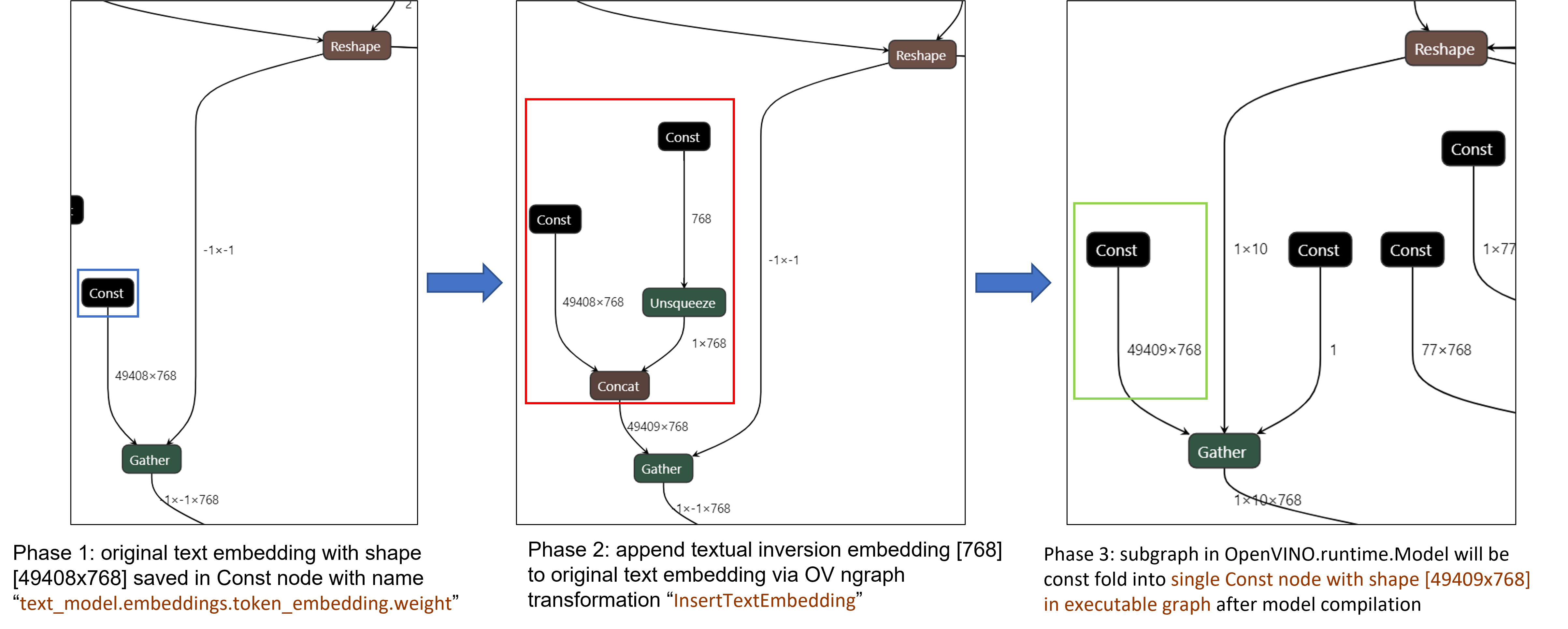
Figure 4. 3 phase of SD 1.5 text encoder subgraph with single textual inversion visualized in Netron.

As Figure 4 shows, In the first phase, the original text embedding (marked as blue rectangle) is saved in Const node “text_model.embeddings.token_embedding.weight” with shape [49408,768], after InsertTextEmbedding ngraph transformation, new subgraph (marked as red rectangle) will be created in 2nd phase. In the 3rd phase, during model compilation, the new subgraph will be const folding into a single const node (marked as green rectangle) with a new shape [49409,768] by OpenVINO^TM ConstantFolding transformation.

Stable Diffusion Textual Inversion Sample

Here are textual inversion examples verified with Stable Diffusion v1.5, Stable Diffusion v2.1 and Stable Diffusion XL 1.0 Base pipeline with latest optimum-intel

Setup Environment

conda create -n optimum-intel python=3.10
conda activate optimum-intel
python -m pip install "optimum-intel[openvino]"@git+https://github.com/huggingface/optimum-intel.git
python -m pip install transformers, diffusers, safetensors
python -m pip install invisible-watermark>=0.2.0

Run SD 1.5 + Cat-Toy Textual Inversion Example

from optimum.intel import OVStableDiffusionPipeline
import numpy as np

model_id = "runwayml/stable-diffusion-v1-5"
prompt = "A <cat-toy> back-pack"
np.random.seed(42)

# Run pipeline without textual inversion
pipe = OVStableDiffusionPipeline.from_pretrained(model_id, compile=False)
pipe.compile()
image1 = pipe(prompt, num_inference_steps=50).images[0]
image1.save("sd_v1.5_without_cat_toy_ti.png")

# Run pipeline with textual inversion
pipe.clear_requests()
pipe.load_textual_inversion("sd_concepts/cat-toy", "<cat-toy>")
pipe.compile()
image2 = pipe(prompt, num_inference_steps=50).images[0]
image2.save("sd_v1.5_with_cat_toy_ti.png")

Figure 5. The left image shows the generation result of SD 1.5 baseline, while the right image shows the generation result of SD 1.5 baseline + Cat-Toy textual inversion.

Run SD 2.1 + Midjourney 2.0 Textual Inversion Example

from optimum.intel import OVStableDiffusionPipeline
import numpy as np

model_id = "stabilityai/stable-diffusion-2-1"
prompt = "A <midjourney> style photo of an astronaut riding a horse on mars"
np.random.seed(42)

# Run pipeline without midjourney textual inversion
pipe = OVStableDiffusionPipeline.from_pretrained(model_id, compile=False, cache_dir=None)
pipe.compile()
image1 = pipe(prompt, num_inference_steps=50).images[0]
image1.save("sd_v2.1_without_midjourney_ti.png")

# Run pipeline with midjourney textual inversion
pipe.clear_requests()
pipe.load_textual_inversion("midjourney_sd_2_0", "<midjourney>")
pipe.compile()
image2 = pipe(prompt, num_inference_steps=50).images[0]
image2.save("sd_v2.1_with_midjourney_ti.png")

Figure 6. The left image shows the generation result of SD 2.1 baseline, while the right image shows the generation result of SD 2.1 + Midjourney 2.0 textual inversion.

Run SDXL 1.0 Base + CharTurnerV2 Textual Inversion Example

from optimum.intel import OVStableDiffusionXLPipeline
import numpy as np

model_id = "stabilityai/stable-diffusion-xl-base-1.0"
prompt = "charturnerv2, multiple views of the same character in the same outfit, a character turnaround of a beautiful woman wearing a red jacket and black shirt, best quality, intricate details."
np.random.seed(112)

pipe = OVStableDiffusionXLPipeline.from_pretrained(model_id, export=False, compile=False, cache_dir=None)

# Run pipeline without textual inversion
pipe.compile()
image1 = pipe(prompt, num_inference_steps=50).images[0]
image1.save("sdxl_base_1.0_without_charturnerv2_ti.png")

# Run pipeline with textual inversion
pipe.clear_requests()
pipe.load_textual_inversion("./charturnerv2.pt", "charturnerv2")
pipe.compile()
image2 = pipe(prompt, num_inference_steps=50).images[0]
image2.save("sdxl_base_1.0_with_charturnerv2_ti.png")

Figure 7. The left image shows the generation result of SDXL 1.0 Base baseline, while the right image shows the generation result of SDXL 1.0 Base + CharTurnerV2 textual inversion.

Conclusion

In this blog, we proposed to load textual inversion embedding in the stable diffusion pipeline in runtime to save disk storage while keeping flexibility.

Implemented OVTextualInversionLoaderMixin to update tokenizer with additional token id and update text encoder with InsertTextEmbedding OpenVNO ngraph transformation.
Provides sample code to load textual inversion with SD 1.5, SD 2.1, and SDXL 1.0 Base and inference with Optimum-Intel

‍

Reference

An Image is Worth One Word: Personalizing Text-to-Image Generation using Textual Inversion

Optimum-Intel Text-to-Image with Textual Inversion

Hugging Face Textual Inversion

Apply dynamic LoRA into Stable Diffusion v1.5 with OpenVINO

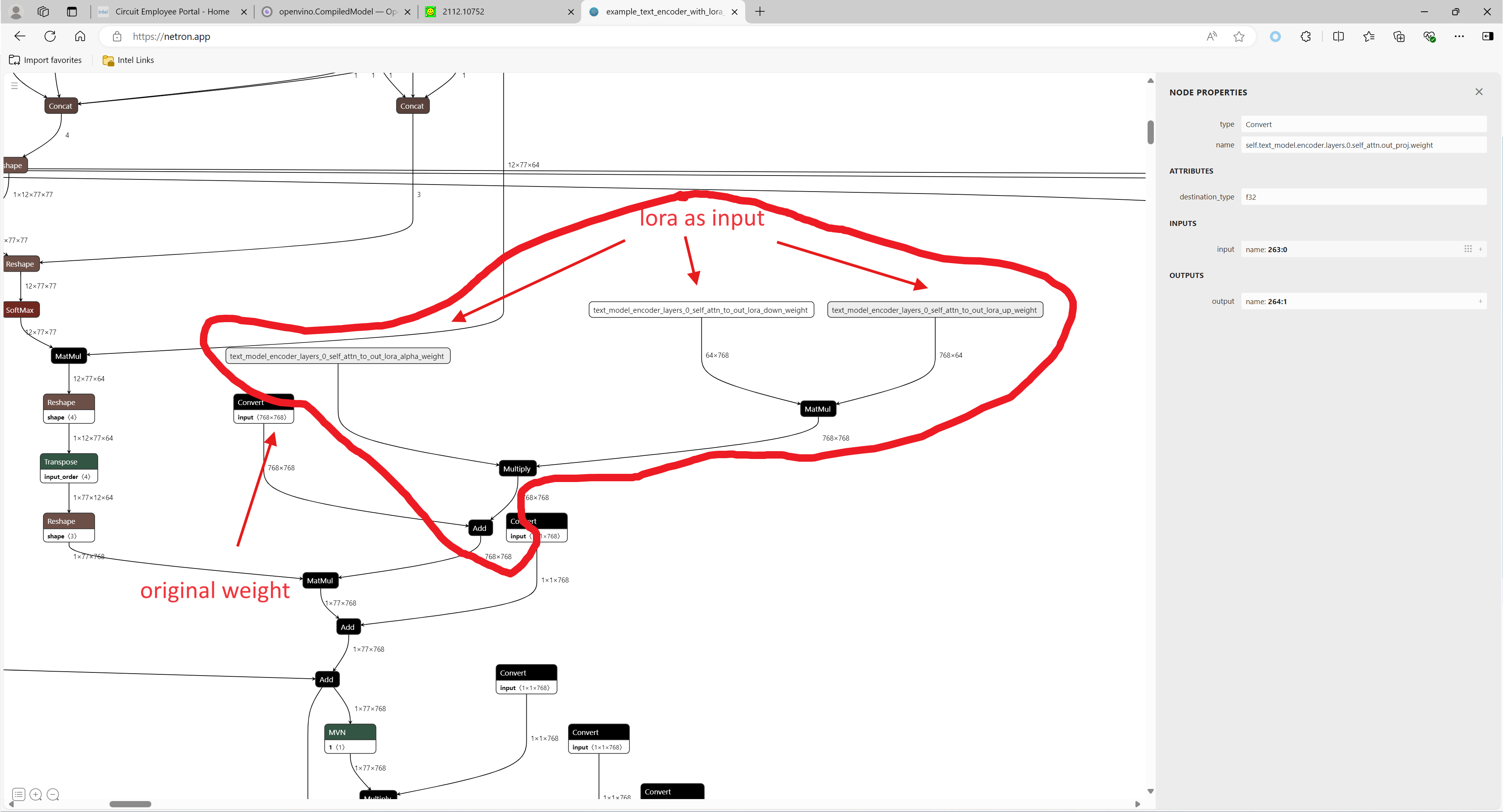
LoRA, or Low-Rank Adaptation, reduces the number of trainable parameters by learning pairs of rank-decompostion matrices while freezing the original weights. This vastly reduces the storage requirement for large language models adapted to specific tasks and enables efficient task-switching during deployment all without introducing inference latency. Thus for a basic large model, the task scenarios of the model can be changed by different LoRAs. In a previous blog, it has been described how to convert the LoRAs-fused base model from pytorch to OpenVINO IR, but this method has the shortcoming of not being able to dynamically switch between LoRAs, which happen to be famous for their flexibility.

This blog will introduce how to implement the dynamic switching of LoRAs in a trick way. Specifically, for most of the tasks, the structure of the base model and LoRAs is unchanged, what changes is the task-specific LoRAs weights, and we can use these LoRAs weights as inputs to the model to achieve the dynamic switching function. All the code involved in this blog can be found here.

‍

‍

1. Environment preparation

# %python -m venv stable-diffusion-lora
# %source stable-diffusion-lora/bin/activate
git clone https://github.com/TianmengChen/sd1.5_controlnet_lora.git
pip install -r requirements.txt

‍

2. Convert and inference

you should first change the lora file path and configs at first around line 478 in ov_model_export.py, after run python ov_model_ export.py, you will get related OpenVINO IR model. Then you can run ov_model_infer.py.

python ov_model_export.py
python ov_model_infer.py

‍

3. Codes explanation

The most important part is the code in util.py, which is used to modify the model graph and load lora.

Function load_lora(lora_path, DEVICE_NAME) is used to load lora, get lora's shape and weights per layers and modify each layer's name.

‍

def load_lora(lora_path, DEVICE_NAME):
    state_dict = load_file(lora_path)
    if DEVICE_NAME =="CPU":
        for key, value in state_dict.items():
            if isinstance(value, torch.Tensor):
                    value_fp32 = value.type(torch.float32)
                    state_dict[key] = value_fp32

    layers_per_block = 2#TODO
    state_dict = _maybe_map_sgm_blocks_to_diffusers(state_dict, layers_per_block)
    state_dict, network_alphas = _convert_non_diffusers_lora_to_diffusers(state_dict)

    # now keys in format like: "unet.up_blocks.0.attentions.2.transformer_blocks.8.ff.net.2.lora.down.weight"'
    new_state_dict = {}
    for key , value in state_dict.items():
        if len(value.shape)==4:
            # new_value = torch.reshape(value, (value.shape[0],value.shape[1]))
            new_value = torch.squeeze(value)
        else:
            new_value = value
        new_state_dict[key.replace('.', '_').replace('_processor','')] = new_value
    # now keys in format like: "unet_up_blocks_0_attentions_2_transformer_blocks_8_ff_net_2_lora_down_weight"'

    LORA_PREFIX_UNET = "unet"
    LORA_PREFIX_TEXT_ENCODER = "text_encoder"
    LORA_PREFIX_TEXT_2_ENCODER = "text_encoder_2"

    lora_text_encoder_input_value_dict = {}
    lora_text_encoder_2_input_value_dict = {}
    lora_unet_input_value_dict = {}

    lora_alpha = collections.Counter(network_alphas.values()).most_common()[0][0]

    for key in new_state_dict.keys():
        if LORA_PREFIX_TEXT_ENCODER in key and "lora_down" in key and LORA_PREFIX_TEXT_2_ENCODER not in key:
            layer_infos = key.split(LORA_PREFIX_TEXT_ENCODER + "_")[-1]
            lora_text_encoder_input_value_dict[layer_infos] = new_state_dict[key]
            lora_text_encoder_input_value_dict[layer_infos.replace("lora_down", "lora_up")] = new_state_dict[key.replace("lora_down", "lora_up")]

        elif LORA_PREFIX_TEXT_2_ENCODER in key and "lora_down" in key:
            layer_infos = key.split(LORA_PREFIX_TEXT_2_ENCODER + "_")[-1]
            lora_text_encoder_2_input_value_dict[layer_infos] = new_state_dict[key]
            lora_text_encoder_2_input_value_dict[layer_infos.replace("lora_down", "lora_up")] = new_state_dict[key.replace("lora_down", "lora_up")]

        elif LORA_PREFIX_UNET in key and "lora_down" in key:
            layer_infos = key.split(LORA_PREFIX_UNET + "_")[-1]
            lora_unet_input_value_dict[layer_infos] = new_state_dict[key]
            lora_unet_input_value_dict[layer_infos.replace("lora_down", "lora_up")] = new_state_dict[key.replace("lora_down", "lora_up")]

    #now the keys in format without prefix

    return lora_text_encoder_input_value_dict, lora_text_encoder_2_input_value_dict, lora_unet_input_value_dict, lora_alpha

‍

Function add_param(model, lora_input_value_dict) is used to add input parameter per names of related layers, which will be connected to model with manager.register_pass(InsertLoRAUnet(input_param_dict)) and manager.register_pass(InsertLoRATE(input_param_dict)), in these two classes, we search the whole model graph to find the related layers by their names and connect them with lora.

def add_param(model, lora_input_value_dict):
        param_list = []
        for key, value in lora_input_value_dict.items():
            if '_lora_down' in key:
                key_down = key
                key_up = key_down.replace('_lora_down','_lora_up')
                name_alpha = key_down.replace('_lora_down','_lora_alpha')
                lora_alpha = ops.parameter(shape='',name=name_alpha)
                lora_alpha.output(0).set_names({name_alpha})
                # lora_down = ops.parameter(shape=[-1, lora_input_value_dict[key_down].shape[-1]], name=key_down)
                lora_down = ops.parameter(shape=lora_input_value_dict[key_down].shape, name=key_down)
                lora_down.output(0).set_names({key_down})
                # lora_up = ops.parameter(shape=[lora_input_value_dict[key_up].shape[0], -1], name=key_up)
                lora_up = ops.parameter(shape=lora_input_value_dict[key_up].shape, name=key_up)
                lora_up.output(0).set_names({key_up})
                param_list.append(lora_alpha)
                param_list.append(lora_down)
                param_list.append(lora_up)
        model.add_parameters(param_list)

‍

class InsertLoRAUnet(MatcherPass):
    def __init__(self, input_param_dict):
        MatcherPass.__init__(self)
        self.model_changed = False
        param = WrapType("opset10.Convert")

        def callback(matcher: Matcher) -> bool:
            root = matcher.get_match_root()
            root_output = matcher.get_match_value()
            for key in input_param_dict.keys():
                if root.get_friendly_name().replace('.','_').replace('self_unet_','') == key.replace('_lora_down','').replace('to_out','to_out_0'):

                    key_down = key
                    key_up = key_down.replace('_lora_down','_lora_up')
                    key_alpha = key_down.replace('_lora_down','_lora_alpha')

                    consumers = root_output.get_target_inputs()

                    lora_up_node = input_param_dict.pop(key_up)
                    lora_down_node = input_param_dict.pop(key_down)
                    lora_alpha_node = input_param_dict.pop(key_alpha)   

                    lora_weights = ops.matmul(data_a=lora_up_node, data_b=lora_down_node, transpose_a=False, transpose_b=False, name=key.replace('_down',''))
                    lora_weights_alpha = ops.multiply(lora_alpha_node, lora_weights)
                    if len(root.shape)!=len(lora_weights_alpha.shape):
                        # lora_weights_alpha_reshape = ops.reshape(lora_weights_alpha, root.shape, special_zero=False)
                        lora_weights_alpha_reshape = ops.unsqueeze(lora_weights_alpha, axes=[2, 3])
                        add_lora = ops.add(root,lora_weights_alpha_reshape,auto_broadcast='numpy')
                    else:
                        add_lora = ops.add(root,lora_weights_alpha,auto_broadcast='numpy')
                    for consumer in consumers:
                        consumer.replace_source_output(add_lora.output(0))

                    return True
            # Root node wasn't replaced or changed
            return False
        
        self.register_matcher(Matcher(param,"InsertLoRAUnet"), callback)

‍

class InsertLoRATE(MatcherPass):
    def __init__(self, input_param_dict):
        MatcherPass.__init__(self)
        self.model_changed = False
        param = WrapType("opset10.Convert")

        def callback(matcher: Matcher) -> bool:
            root = matcher.get_match_root()
            root_output = matcher.get_match_value()
            root_name = None
            if 'Constant_' in root.get_friendly_name() and root.shape == ov.Shape([768,768]):
                target_input = root.output(0).get_target_inputs()
                for v in target_input:
                    for input_of_MatMul in v.get_node().inputs():
                        if input_of_MatMul.get_shape()== ov.Shape([1,77,768]):
                            Add_Node = input_of_MatMul.get_source_output().get_node()
                            for Add_Node_output in Add_Node.output(0).get_target_inputs():
                                if 'k_proj' in Add_Node_output.get_node().get_friendly_name():
                                    for i in Add_Node_output.get_node().inputs():
                                        if i.get_shape() == ov.Shape([768,768]) and 'k_proj' in i.get_source_output().get_node().get_friendly_name():
                                            root_name = i.get_source_output().get_node().get_friendly_name().replace('k_proj', 'q_proj')

            root_friendly_name = root_name if root_name else root.get_friendly_name()
            
            for key in input_param_dict.keys():
                if root_friendly_name.replace('.','_').replace('self_','') == key.replace('_lora_down','_proj').replace('_to','').replace('_self',''):
                    # print(root_friendly_name)
                    key_down = key
                    key_up = key_down.replace('_lora_down','_lora_up')
                    key_alpha = key_down.replace('_lora_down','_lora_alpha')

                    consumers = root_output.get_target_inputs()

                    lora_up_node = input_param_dict.pop(key_up)
                    lora_down_node = input_param_dict.pop(key_down)
                    lora_alpha_node = input_param_dict.pop(key_alpha)   

                    lora_weights = ops.matmul(data_a=lora_up_node, data_b=lora_down_node, transpose_a=False, transpose_b=False, name=key.replace('_down',''))
                    lora_weights_alpha = ops.multiply(lora_alpha_node, lora_weights)
                    add_lora = ops.add(root,lora_weights_alpha,auto_broadcast='numpy')
                    for consumer in consumers:
                        consumer.replace_source_output(add_lora.output(0))

                    return True
                
            if len(input_param_dict) == 0:
                print("All loras are added")
            # Root node wasn't replaced or changed
            return False
        
        self.register_matcher(Matcher(param,"InsertLoRATE"), callback)

‍

4. GenAI

In addition to this, the latest OpenVINO GenAI provides the Cpp API for LoRA. You can find it here.

‍

Stable Diffusion

Dynamic shapes support in OpenVINO JIT compiler boosts inference performance by 40%

Introduction

Architecture

Lowering Pipeline

Dynamic Shapes Support

Results

Performance Improvements

Memory Consumption Improvements

Conclusion

References

Notices & Disclaimers

OpenVINO Latent Consistency Model C++ pipeline with LoRA model support

Introduction

Model Conversion

LCM model

Tokenizer

Conversion step

C++ Pipeline

Pipeline flow

LoRA support

Build and Run LCM demo

See Also

C++ Pipeline for Stable Diffusion v1.5 with Pybind for Lora Enabling

Authors: Fiona Zhao, Xiake Sun, Su Yang

Step 1: Prepare Environment

Setup in Linux:

Step 2: Prepare SD model and Tokenizer Model

Step 3: Build Pipeline

Step 4: Run Pipeline

Benchmark:

Limitation:

Setup in Windows 10 with VS2019:

1. Python env: Setup Conda env SD-CPP with the anaconda prompt terminal

2. C++ dependencies:

3. Setup of conda env SD-CPP and Setup OpenVINO with setupvars.bat

4. CMake with build.bat like:

5. Setup of Visual Studio with release and x64, and build: open .sln file in the build Dir

6. Run the SD_generate.exe

Enable Textual Inversion with Stable Diffusion Pipeline via Optimum-Intel

Introduction

How to enable textual inversion in runtime?

Stable Diffusion Textual Inversion Sample

Setup Environment

Run SD 1.5 + Cat-Toy Textual Inversion Example

Run SD 2.1 + Midjourney 2.0 Textual Inversion Example

Run SDXL 1.0 Base + CharTurnerV2 Textual Inversion Example

Conclusion

Reference

Apply dynamic LoRA into Stable Diffusion v1.5 with OpenVINO

1. Environment preparation

2. Convert and inference

3. Codes explanation

4. GenAI