AI-pipeline

Authors: Hongbo Zhao, Fiona Zhao, Tong Qiu

Why Choose the Ollama + OpenVINO Combination?

Dual-Engine Driven Technical Advantages

The integration of Ollama and OpenVINO delivers a powerful dual-engine solution for the management and inference of large language models (LLMs). Ollama offers a streamlined model management toolchain, while OpenVINO provides efficient acceleration capabilities for model inference across Intel hardware (CPU/GPU/NPU). This combination not only simplifies the deployment and invocation of models but also significantly enhances inference performance, making it particularly suitable for scenarios demanding high performance and ease of use.

You can find more information on github repository:

https://github.com/openvinotoolkit/openvino_contrib/tree/master/modules/ollama_openvino

Core Value of Ollama

    1. Streamlined LLM Management Toolchain: Ollama provides a user-friendly command-line interface, enabling users to effortlessly download, manage, and run various LLM models.

    2. One-Click Model Deployment: With simple commands, users can quickly deploy and invoke models without complex configurations.

    3. Unified API Interface: Ollama offers a unified API interface, making it easy for developersto integrate into various applications.

    4. Active Open-Source Community: Ollama boasts a vibrant open-source community, providing users with abundant resources and support.

Limitations of Ollama

Currently, Ollama only supports llama.cpp as itsbackend, which presents some inconveniences:

    1. Limited Hardware Compatibility: llama.cpp is primarily optimized for CPUs and NVIDIA GPUs, and cannot fully leverage the acceleration capabilities of Intel GPUs or NPUs, resulting in suboptimal performance in high-performance computing scenarios.

    2. Performance Bottlenecks: For large-scale models or high-concurrency scenarios, the performance of llama.cpp may fall short, especially when handling complex tasks, leading to slower inference speeds.

Breakthrough Capabilities of OpenVINO

    1. Deep Optimization for Intel Hardware (CPU/iGPU/Arc dGPU/NPU): OpenVINO is deeply optimized for Intel hardware, fully leveraging the performance potential of CPUs, iGPUs, dGPUs, and NPUs.

    2. Cross-Platform Heterogeneous Computing Support: OpenVINO supports cross-platform heterogeneous computing, enabling efficient model inference across different hardware platforms.

    3. Model Quantization and Compression Toolchain: OpenVINO provides a comprehensive toolchain for model quantization and compression, significantly reducing model size and improving inference speed.

    4. Significant Inference Performance Improvement: Through OpenVINO's optimizations, model inference performance can be significantly enhanced, especially for large-scale models and high-concurrency scenarios.

    5. Extensibility and Flexibility Support: OpenVINO GenAI offers robust extensibility and flexibility for Ollama-OV, supporting pipeline optimization techniques such as speculative decoding, prompt-lookup decoding, pipeline parallelization, and continuous batching, laying a solid foundation for future pipeline serving optimizations.

Developer Benefits of Integration

    1. Simplified Development Experience: Retains Ollama's CLI interaction features, allowing developers to continue using familiar command-line tools for model management and invocation.

    2. Performance Leap: Achieves hardware-level acceleration through OpenVINO, significantly boosting model inference performance, especially for large-scale models and high-concurrency scenarios.

    3. Multi-Hardware Adaptation and Ecosystem Expansion: OpenVINO's support enables Ollama to adapt to multiple hardware platforms, expanding its application ecosystem and providing developers with more choices and flexibility.

Three Steps to Enable Acceleration

    1. Download Precompiled Executables

       please refer to : https://github.com/zhaohb/ollama_ov/tree/main?tab=readme-ov-file#google-driver

    2.Configure OpenVINO GenAI Environment

        For Windows systems, first extract the downloaded OpenVINO GenAI package to the directory openvino_genai_windows_2025.2.0.0.dev20250320_x86_64, then execute the following commands:

cd openvino_genai_windows_2025.2.0.0.dev20250320_x86_64
setupvars.bat

    3. Set Up cgocheck

      Windows:

           set GODEBUG=cgocheck=0

      Linux:

          export GODEBUG=cgocheck=0

At this point, the executable files have been downloaded, and the OpenVINO GenAI, OpenVINO, and CGO environments have been successfully configured.

Custom Model Deployment Guide

Since the Ollama Model Library does not support uploading non-GGUF format IR models, we will create an OCI image locally using OpenVINO IR that is compatible with Ollama. Here, we use the DeepSeek-R1-Distill-Qwen-7B model as an example:

    1. Download the OpenVINO IR Model

        Download the model from ModelScope:

pip install modelscope
modelscope download --model zhaohb/DeepSeek-R1-Distill-Qwen-7B-int4-ov --local_dir ./DeepSeek-R1-Distill-Qwen-7B-int4-ov

    2. Package the Downloaded OpenVINO IR Directory

        Compress the directory into a *.tar.gz file:

tar -zcvf DeepSeek-R1-Distill-Qwen-7B-int4-ov.tar.gz DeepSeek-R1-Distill-Qwen-7B-int4-ov

    3. Create a Modelfile

        Define the model configuration in a Modelfile:

FROM DeepSeek-R1-Distill-Qwen-7B-int4-ov.tar.gz
ModelType "OpenVINO"
InferDevice "GPU"
PARAMETER stop ""
PARAMETER stop "```"
PARAMETER stop "</User|>"
PARAMETER stop "<|end_of_sentence|>"
PARAMETER stop "</｜"
PARAMETER max_new_token 4096
PARAMETER stop_id 151643
PARAMETER stop_id 151647
PARAMETER repeat_penalty 1.5
PARAMETER top_p 0.95
PARAMETER top_k 50
PARAMETER temperature 0.8

    4. Create an Ollama-Compatible Model

        Use the Modelfile to create a model supported by Ollama:

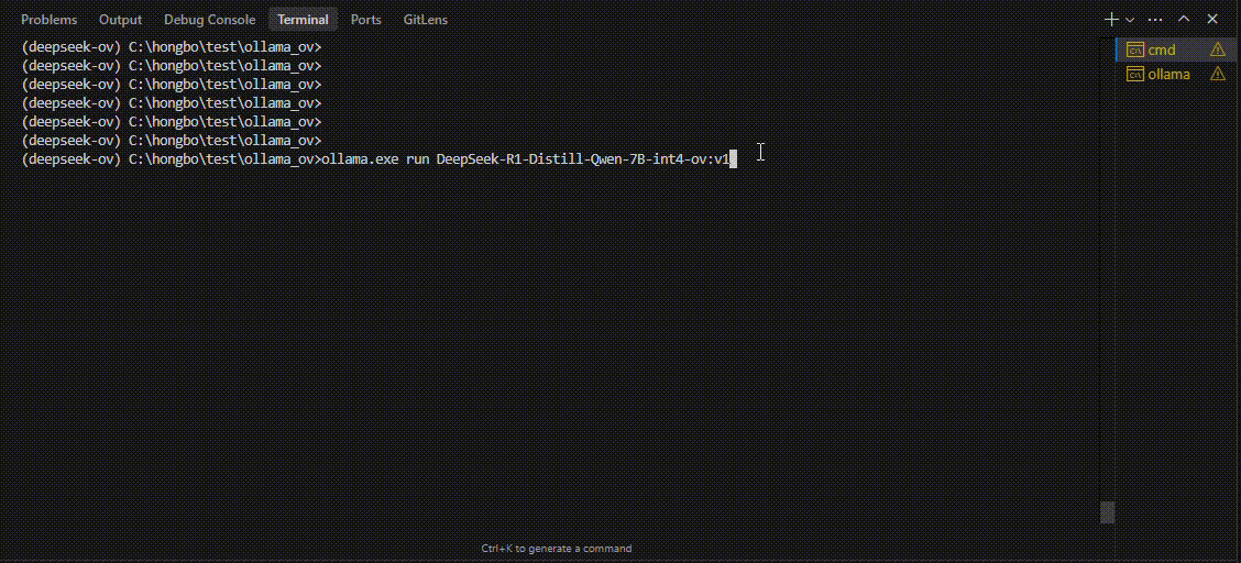
ollama create DeepSeek-R1-Distill-Qwen-7B-int4-ov:v1 -f Modelfile

‍

With these steps, we have successfully created the DeepSeek-R1-Distill-Qwen-7B-int4-ov:v1 model, which is now ready for use with the Ollama OpenVINO backend.

1. Introduction

Janus is a unified multimodal understanding and generation model developed by DeepSeek. Janus proposed decoupling visual encoding to alleviate the conflict between multimodal understanding and generation tasks. Janus-Pro further scales up the Janus model to larger model size (deepseek-ai/Janus-Pro-1B &  deepseek-ai/Janus-Pro-7B) with optimized training strategy and training data, achieving significant advancements in both multimodal understanding and text-to-image tasks.

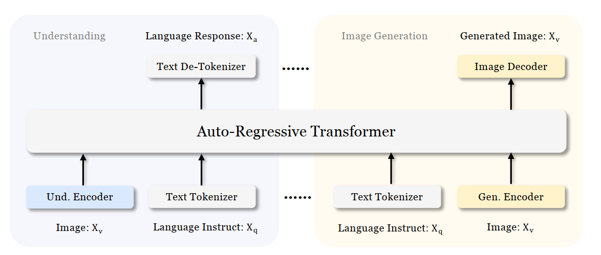
Figure 1 shows the architecture of Janus-Pro, which decouples visual encoding for multimodal understanding and visual generation. “Und. Encoder” and “Gen. Encoder” are abbreviations for “Understanding Encoder” and “Generation Encoder”.  For the multimodal understanding task, SigLIP vision encoder used to extract high-dimensional semantic features from the image, while for the vision generation task, VQ tokenizer used to map images to discrete IDs. Both the understanding adaptor and the generation adaptor are two-layer MLPs to map the embeddings to the input space of LLM.

In this blog, we will introduce how to deploy Janus-Pro model with OpenVINO^TM runtime on the intel platform.

2. Janus-Pro Pytorch Model to OpenVINO^TM Model Conversion

2.1. Setup Python Environment

$ git clone https://github.com/sammysun0711/openvino_aigc_samples.git
$ cd openvino_aigc_samples/Janus
$ conda create -n janus-ov python=3.10
$ conda activate janus-ov
$ pip install -r requirements.txt

2.2 Download Janus Pytorch model (Optional)

$ modelscope download --model deepseek-ai/Janus-Pro-1B --local_dir Janus-Pro-1B

2.3. Convert Pytorch Model to OpenVINO^TM INT4 Model

$ python convert_janus.py -m Janus-Pro-1B -o Janus-Pro-1B-OV

The converted OpenVINO will be saved in Janus-Pro-1B-OV directory for deployment.

3.  Janus-Pro Inference with OpenVINO^TM Demo

In this section, we provide several examples to show Janus-Pro for multimodal understanding and vision generation tasks.

3.1. Multimodal Understanding Task – Image Caption with OpenVINO^TM

$ python run_janus_vlm_ov.py -m Janus-Pro-1B-OV -p "Describe image in det
ails" -i images/cat_in_box.png -d GPU

Prompt: Describe image in details

Input image:

Generated Output:

The image shows a gray tabby cat lying inside an open cardboard box on a carpeted floor. The cat is lying on its back with its belly exposed, looking relaxed and comfortable. The background includes a beige-colored sofa and a light-colored curtain,
 suggesting a cozy indoor setting. The cat's tail is curled around its body, and it appears to be enjoying itself.

3.2. Multimodal Understanding Task – Equation Description with OpenVINO^TM

$ python run_janus_vlm_ov.py -m Janus-Pro-1B-OV -p "Generate the latex code of this formula" -i images/equation.png -d GPU

Prompt: Generate the latex code of this formula

Input Image:

Generated Output:

\[ A_n = a_0 \begin{bmatrix} 1 & + \frac{3}{4} \sum_{k=1}^{n} \begin{bmatrix} 4 \\ 9 \end{bmatrix}^k \end{bmatrix} \]

This formula represents the cumulative sum of the first \( n \) terms of the sequence \( a_n \), where \( a_n \) is the sequence of \( a_0 \), \( \frac{3}{4} \), and \( \begin{bmatrix} 4 \\ 9 \end{bmatrix}^k \). The first term \( a_0 \) is the first term of the sequence, the second term is the sum of the first \( n-1 \) terms, and the third term is the sum of the first \( n \) terms. The sequence \( \begin{bmatrix} 4 \\ 9 \end{bmatrix}^k \) represents the \( k \)-th term of the sequence. The
 formula calculates the cumulative sum of the sequence \( a_n \).

This formula can be used to calculate the cumulative sum of the sequence \( a_n \) for any given \( n \).

3.3. Multimodal Understanding Task – Code Generation with OpenVINO^TM

$ python run_janus_vlm_ov.py -m Janus-Pro-1B-OV -p "Generate the matplotlib pyplot code for this plot" -i images\pie_chart.png -d GPU

Prompt: Generate the matplotlib pyplot code for this plot

Input Image:

Generated Output:

The attention mask is not set and cannot be inferred from input because pad token is same as eos token. As a consequence, you may observe unexpected behavior. Please pass your input's `attention_mask` to obtain reliable results.
Sure, here is the code to generate the matplotlib plot based on the information in the image:

```python
import matplotlib.pyplot as plt

# Data
data = {
    'Hogs': 30,
    'Frogs': 15,
    'Logs': 10,
    'Dogs': 45
}

# Create the plot
plt.figure(figsize=(10, 6))

# Pie chart
for key, value in data.items():
    # Calculate the percentage of the pie chart
    percentage = value / 100

    # Add the pie slice
    plt.pie(percentage, labels=data.keys(), autopct='%1.1f%%')

# Title and labels
plt.title('Pie chart')
plt.xlabel('Categories')
plt.ylabel('Percentage')

# Show the plot
plt.show()
```

This code will create a pie chart based on the data provided in the image.

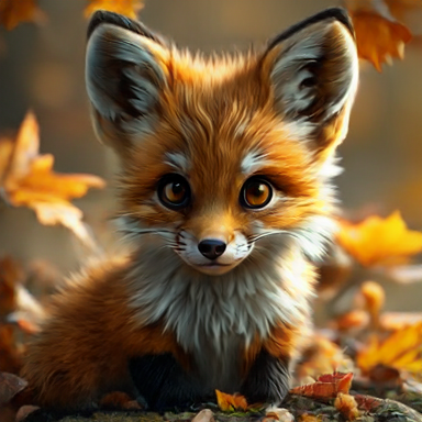
3.4. Vision Generation Task with OpenVINO^TM

$ python run_janus_t2i_ov.py -m Janus-Pro-1B-OV -d GPU

Input Prompt: A cute and adorable baby fox with big brown eyes, autumn leaves in the background enchanting, immortal, fluffy, shiny mane, Petals, fairyism, unreal engine 5 and Octane Render, highly detailed, photorealistic, cinematic, natural colors.

Generated image:

4. Performance Evaluation & Memory Usage Analysis

We also provide benchmark scripts to evaluate Janus-Pro model performance and memory usage with OpenVINO^TM inference, you may specify model name and device for your target platform.

4.1. Benchmark Janus-Pro for Multimodal Understanding Task with OpenVINO^TM

$ python benchmark_janus_vlm_ov.py -m Janus-Pro-1B-OV -d GPU

Here are some arguments for benchmark script for Multimodal Understanding Task:

--model_id: specify the Janus OpenVINO^TM model directory

--prompt: specify input prompt for multimodal understanding task

--image_path: specify input image for multimodal understanding task

--niter:  specify number of test iteration, default is 5

--device: specify which device to run inference

--max_new_tokens: specify max number of generated tokens

By default, the benchmark script will run 5 round multimodal understanding tasks on target device, then report pipeline initialization time, average first token latency (including preprocessing), 2^nd+ token throughput and max RSS memory usage.

‍

4.2. Benchmark Janus-Pro for Text-to-Image Task with OpenVINO^TM

$ python benchmark_janus_t2i_ov.py -m Janus-Pro-1B-OV -d GPU

Here are some arguments for benchmark scripts for Text-to-Image Task

--model_id: specify the Janus OpenVINO ^TM model directory

--prompt: specify input prompt for text-to-image generation task

--niter:  specify number of test iteration

--device: specify which device to run inference

By default, the benchmark script will run 5 round image generation tasks on target device, then report the pipeline initialization time, average image generation latency and max RSS memory usage.

‍

5. Conclusion

In this blog, we introduced how to enable Janus-Pro model with OpenVINO^TM runtime, then we demonstrated the Janus-Pro capability for various multimodal understanding and image generation tasks. In the end, we provide python script for performance & memory usage evaluation for both multimodal understanding and image generation task on target platform. 

Authors: Xiake Sun, Su Yang, Tianmeng Chen, Tong Qiu

openvino.genai/samples/cpp/rag_sample at openvino_genai_serving · sammysun0711/openvino.genai (github.com)

OpenVINO GenAI Server (OGS) Update:

-Update LLM: stream generation, reset handle, multi-round chat, model cache config

-Support VLM

-Support Reranker for RAG sample

-Support BLIP image embedding for photo search with DB

-Support C++ GUI with imgui for photo search

Now we scale the text embedding to image embedding for RAG sample and support multi-Vector Retriever for RAG.

1. Multi-Vector Retriever for RAG on text: QA over Document
2. Multi-Vector Retriever for RAG on image: Photo search with DB retrieval

‍

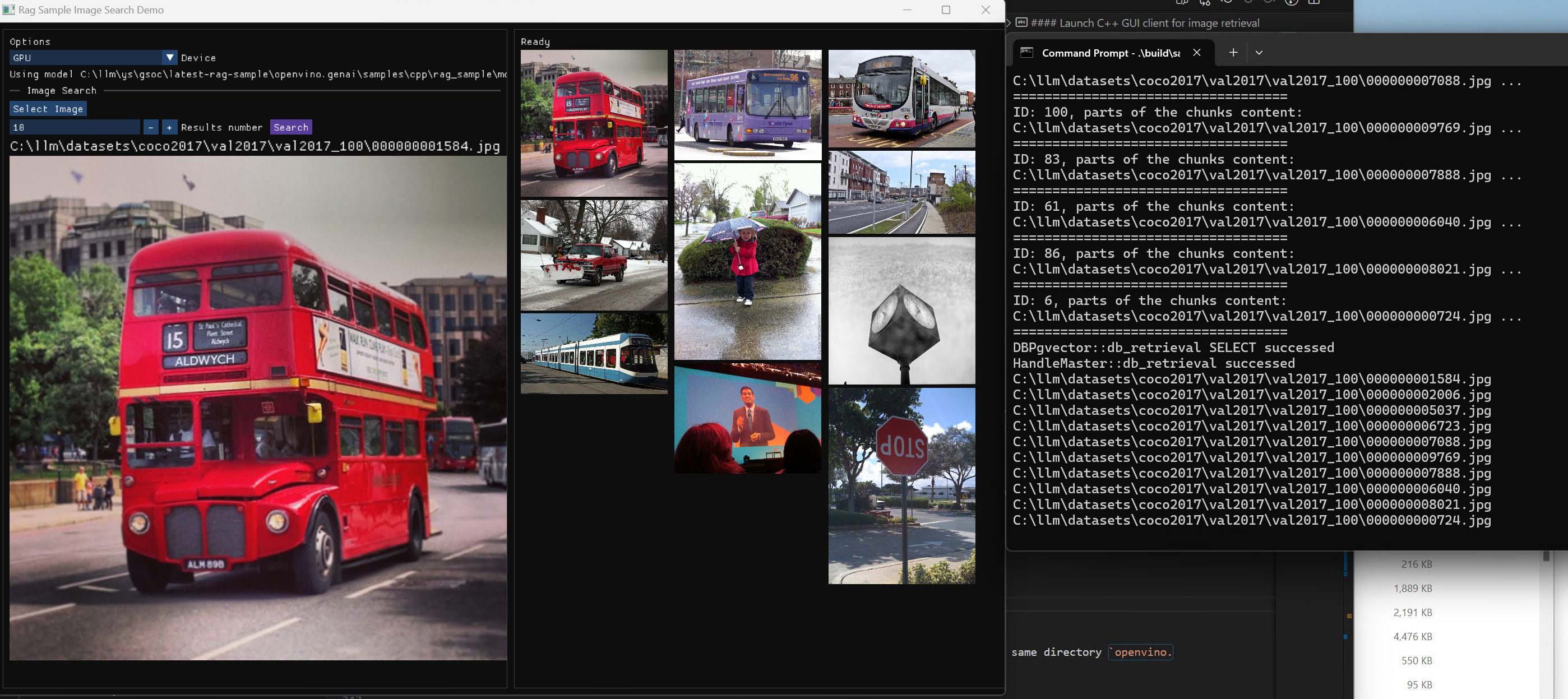
Here is a photo search sample with image embedding.

Usage 2: Photo Search with DB retrieval

Steps:

1.use python client to create image vector DB (PostgreSQL)

2.use GUI to search image

Here is a sample image to demonstrate GUI usage on client platform. we search the bus photo with top 10 similar images from the 100 images which are embedded into Vector DB.

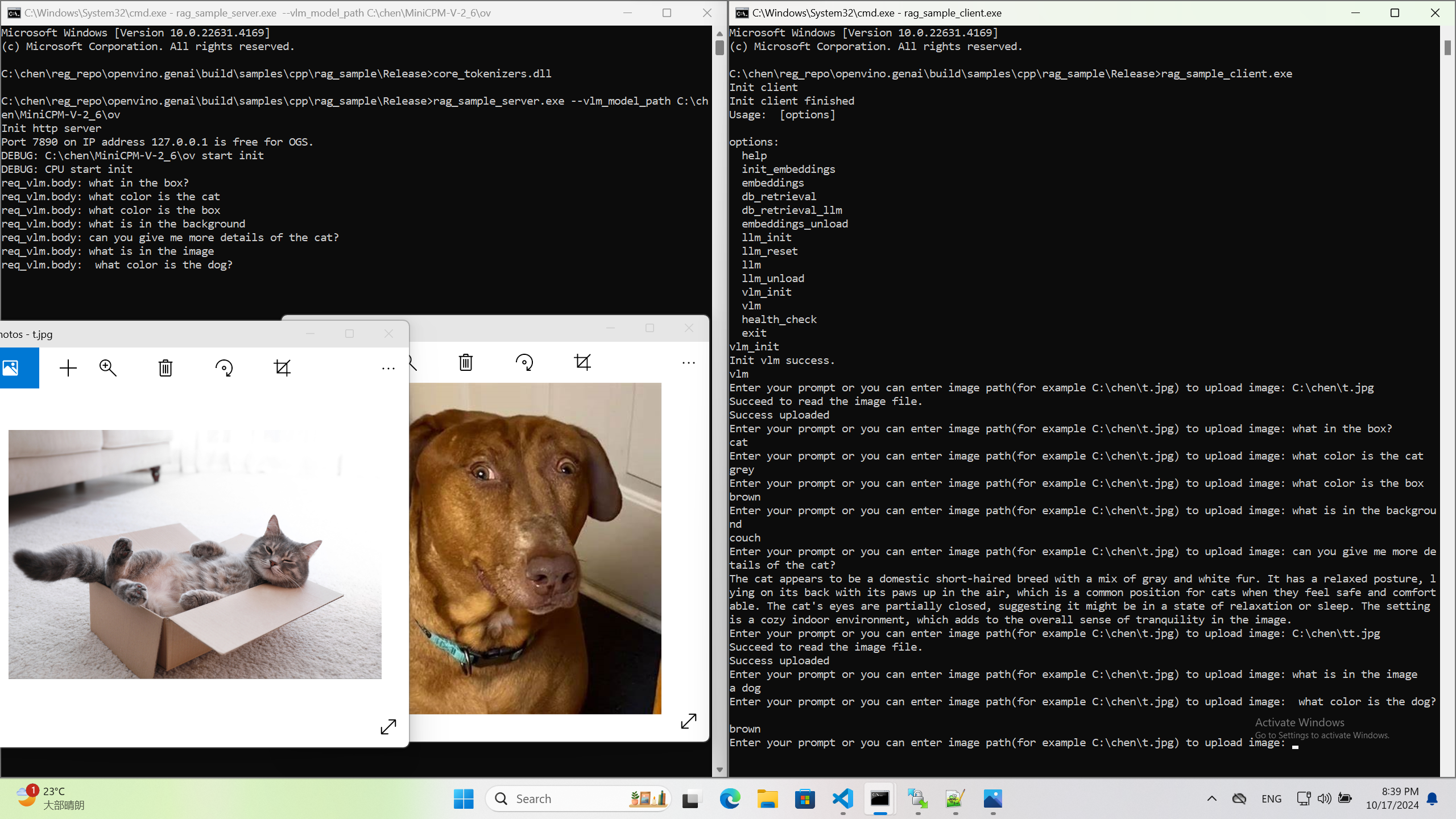
Usage 3: Chat with images via MiniCPM-V

Once we have created a multimodal vector DB through image embedding, we can further communicate with the image through VLM.

We integrate the C++ GenAI sample visual_language_chat with openbmb/MiniCPM-V-2_6.

Here is the demo image on client platform.

‍

Authors: Hongbo Zhao, Fiona Zhao

Introduction

InternVL2.0 is a series of multimodal large language models available in various sizes. The InternVL2-4B model comprises InternViT-300M-448px, an MLP projector, and Phi-3-mini-128k-instruct. It delivers competitive performance comparable to proprietary commercial models across a range of capabilities, including document and chart comprehension, infographics question answering, scene text understanding and OCR tasks, scientific and mathematical problem solving, as well as cultural understanding and integrated multimodal functionalities.

You can find more information on github repository: https://github.com/zhaohb/InternVL2-4B-OV 

OpenVINO^TM backend on InternVL2-4B

Step 1: Install system dependency and setup environment

Create and enable python virtual environment

conda create -n ov_py310 python=3.10 -y
conda activate ov_py310

Clone the InternVL2-4B-OV repository from github

git clonehttps://github.com/zhaohb/InternVL2-4B-OV
cd InternVL2-4B-OV

 Install python dependency

pip install -r requirement.txt
pip install --pre -U openvino openvino-tokenizers --extra-index-url https://storage.openvinotoolkit.org/simple/wheels/nightly

 Step2: Get HuggingFace model

huggingface-cli download --resume-download OpenGVLab/InternVL2-4B --local-dir InternVL2-4B--local-dir-use-symlinks False
cp modeling_phi3.py  InternVL2-4B/modeling_phi3.py
cp modeling_intern_vit.py   InternVL2-4B/modeling_intern_vit.py

 Step 3: Export to OpenVINO™ model

python test_ov_internvl2.py -m ./InternVL2-4B -ov ./internvl2_ov_model -llm_int4_com -vision_int8 -llm_int8_quan -convert_model_only

 Step4: Simple inference test with OpenVINO™

python test_ov_internvl2.py -m ./InternVL2-4B -ov ./internvl2_ov_model -llm_int4_com -vision_int8-llm_int8_quan

 Question: Please describe the image shortly.

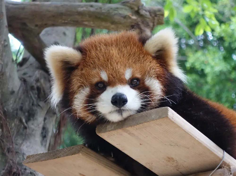
Answer:

The image features a close-up view of a red panda resting on a wooden platform. The panda is characterized by its distinctive red fur, white face, and ears. The background shows a natural setting with green foliage and a wooden structure.

Here are the parameters with descriptions:

python test_ov_internvl2.py --help
usage: Export InternVL2 Model to IR [-h] [-m MODEL_ID] -ov OV_IR_DIR [-d DEVICE] [-pic PICTURE] [-p PROMPT] [-max MAX_NEW_TOKENS] [-llm_int4_com] [-vision_int8] [-llm_int8_quant] [-convert_model_only]
options:
  -h, --help   show this help message and exit  
  -m MODEL_ID, --model_id MODEL_ID   model_id or directory for loading     
  -ov OV_IR_DIR, --ov_ir_dir OV_IR_DIR     output directory for saving model  
  -d DEVICE, --device DEVICE   inference device  
  -pic PICTURE, --picture PICTURE  picture file 
  -p PROMPT, --prompt PROMPT    prompt  
  -max MAX_NEW_TOKENS, --max_new_tokens MAX_NEW_TOKENS    max_new_tokens  
  -llm_int4_com, --llm_int4_compress  llm int4 weight scompress  
  -vision_int8, --vision_int8_quant  vision int8 weights quantize  
  -llm_int8_quant, --llm_int8_quant      llm int8 weights dynamic quantize  
  -convert_model_only, --convert_model_only      convert model to ov only, do not do inference test

Supported optimizations

1. Vision model INT8 quantization and SDPA optimization enabled

2. LLM model INT4 compression

3. LLM model INT8 dynamic quantization

4. LLM model with SDPA optimization enabled

Summary

This blog introduces how to use the OpenVINO™ python API to run the pipeline of the Internvl2-4B model, and uses a variety of acceleration methods to improve the inference speed.

‍

Introduction

moondream2 is a small vision language model designed to run efficiently on edge devices. Although the model has a small number of parameters, it provides high-performance visual processing capabilities. It can quickly understand and process input images and respond to user queries. The model was developed by VikhyatK and is released under the permissive Apache 2.0 license, allowing for commercial use.

You can find more information on github repository: https://github.com/zhaohb/moondream2-ov

OpenVINO^TM backend on moondream2

Step 1: Install system dependency and setup environment

Create and enable python virtual environment

conda create -n ov_py310 python=3.10 -y
conda activate ov_py310

Clone themoondream2-ov repository from gitHub

git clone https://github.com/zhaohb/moondream2-ov
cd moondream2-ov

Install python dependency

pip install -r requirement.txt
pip install --pre -U openvino openvino-tokenizers --extra-index-url https://storage.openvinotoolkit.org/simple/wheels/nightly

Step 2: Get HuggingFace model

git lfs install
git clone https://hf-mirror.com/vikhyatk/moondream2
git checkout 48be9138e0faaec8802519b1b828350e33525d46

Step 3: Export OpenVINO™ models and simple inference test with OpenVINO™

python3 test_ov_moondream2.py -m /path/to/moondream2 -o /path/to/moondream2_ov

Question: Describe this image.

Answer:

The image shows a modern white desk with a laptop, a lamp, and a notebook on it, set against a gray wall and a wooden floor.

‍

Authors :  Qiu Tong, Zhao Hongbo

MeloTTS released by MyShell.ai, is a high-quality, multilingual Text-to-Speech (TTS) library that supports English, Chinese (mixed English), and various other languages. The strengths of the model lie in its lightweight design, which is well-suited for applications on AIPC systems, coupled with its impressive performance. In this article, I will guide you through the process of converting the model to be compatible with OpenVINO toolkits, enabling it to run on various devices such as CPUs, GPUs and NPUs. Additionally, I will provide a concise overview of the model's inference procedure.

‍

Overview of Model Inference Procedure and Pipeline

For each language type, the pipeline requires only two models (two inference procedures). For instance, English language generation necessitates just the 'bert-base-uncased' model and its corresponding MeloTTS-English. Similarly, for Chinese language generation (which includes mixed English), the pipeline needs only the 'bert-base-multilingual-uncased' and MeloTTS-Chinese. This greatly streamlines the pipeline compared to other TTS frameworks, and the compact size of the models makes them suitable for deployment on edge devices.

MeloTTS is based on Variational Inference with adversarial learning for end-to-end Text-to-Speech (VITS). The inference process is illustrated in the figure. It encompasses a text encoder, a stochastic duration predictor, a decoder.

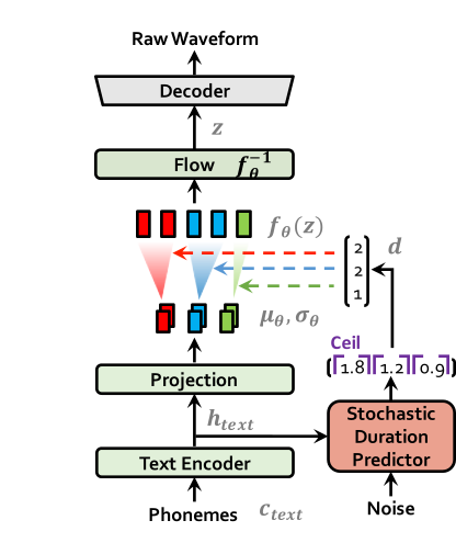
The text encoder accepts phones, tones and a hidden layer from a BERT model as input. It then produces the text encoder's output along with its mean value and a logarithmic variance. To align the input texts with the target speech, the outputs from the encoders are processed using a stochastic duration predictor, which generates an alignment matrix. This matrix is then used to expand the mean value and a logarithmic variance (assuming a Gaussian distribution) to obtain the results for the latent variables .Subsequently, the inverse flow transformation is applied to obtain the distribution of final latent variable z, which represents the spectrogram. In the decoder, by upsampling the spectrogram, the final audio waveform is obtained.

‍

def ov_infer(self, phones=None, phones_length=None, speaker_id=None, tones=None, lang_ids=None, bert=None, ja_bert=None, sdp_ratio=0.2, noise_scale=0.6, noise_scale_w=0.8, speed=1.0):

‍

The inference entry is the function. In practical inference, phone refers to the distinct speech sounds, while tone refers to the vocal pitch contour. For Chinese, a phone corresponds to pinyin, and a tone corresponds to one of the four tones. In English, phones are the consonants and vowels, and tones relate to stress patterns. Here, noise_scale and noise_scale_w do not refer to actual noise. Both noise_scale_w and noise_scale are components within the Stochastic Duration Predictor, used to introduce randomness in order to enhance the expressiveness of the model.

‍

Note that MeloTTS does not include a voice cloning component, unlike the majority of other TTS  models, which makes it more lightweight. If voice cloning is required, please refer to OpenVoice.

‍

Enable Model for OpenVINO

As previously mentioned, the pipeline requires just two models for each language. Taking English as an example, we must first convert both 'bert-base-uncased' and 'MeloTTS-English' into the OpenVINO IR format.

        example_input={
                "x": x_tst,
                "x_lengths": x_tst_lengths,
                "sid": speakers,
                "tone": tones,
                "language": lang_ids,
                "bert": bert,
                "ja_bert": ja_bert,
                "noise_scale": noise_scale,
                "length_scale": length_scale,
                "noise_scale_w": noise_scale_w,
                "sdp_ratio": sdp_ratio,
            }
            
        ov_model = ov.convert_model(
            self.model,
            example_input=example_input,
        )
        get_input_names = lambda: ["phones", "phones_length", "speakers",
                                  "tones", "lang_ids", "bert", "ja_bert",
                                  "noise_scale", "length_scale", "noise_scale_w", "sdp_ratio"]
        for input, input_name in zip(ov_model.inputs, get_input_names()):
            input.get_tensor().set_names({input_name})
        outputs_name = ['audio']
        for output, output_name in zip(ov_model.outputs, outputs_name):
            output.get_tensor().set_names({output_name})
        """
        reshape model
        Set the batch size of all input tensors to 1
        """   
        shapes = {}     
        for input_layer  in ov_model.inputs:
            shapes[input_layer] = input_layer.partial_shape
            shapes[input_layer][0] = 1
        ov_model.reshape(shapes)

        ov.save_model(ov_model, Path(ov_model_path))

‍

For instance, we convert the MeloTTS-English model from the pytorch format directly by utilizing the openvino.convert_model API along with pseudo input data.

Note that the input and output layers (it is optional) are renamed to facilitate subsequent development. Furthermore, the batch dimension for all inputs is fixed at 1, as multiple batches are not required here (this is also optional).

‍

We further quantized both the BERT and TTS models to int8 using pseudo data. We observed that our method of quantizing the TTS model introduces a slight distortion to the current sound. To suppress this, we implemented DeepFilterNet, which is also very lightweight.

‍

More about model conversion and int8 quantization please refer to MeloTTS-OV .

‍

Run BERT part on NPU

To enhance performance and reduce CPU offloading, we can shift the execution of the BERT model to the NPU on Meteor Lake.

To adapt the model for the NPU, we've converted the model to accept static shape inputs a and pad each input during inference.

def reshape_for_npu(model, bert_static_shape = 32):
        # change dynamic shape to static shape
        shapes = dict()
        for input_layer  in model.inputs:
            shapes[input_layer] = bert_static_shape
        model.reshape(shapes)
        ov.save_model(model, Path(ov_model_save_path))
        print(f"save static model in {Path(ov_model_save_path)}")

def main():
    core = Core()
    model = core.read_model(ov_model_path)
    reshape_for_npu(model, bert_static_shape=bert_static_shape)

‍

Simple Demo

Here are the audio files generated by the int8 quantized model from OpenVINO.

https://github.com/zhaohb/MeloTTS-OV/tree/speech-enhancement-and-npu/demo

‍

‍

‍

Authors: Tianmeng Chen, Xiake Sun, Fiona Zhao, Su Yang

Introduction

Personalized Speech Synthesis is the process of using some recording devices around you to record certain voice clips of a particular person, and then letting Text-To-Speech (TTS) technology synthesize the voice, manner of speaking, and emotion of a particular person.  SAMBERT-HifiGAN is a complete personalized TTS solution designed by Alibaba Damo Institute, which includes the first part of SAMBERT's acoustic model and the second part of the HifiGAN vocoder.

In this blog, we will introduce how to utilize OpenVINO^TM Python API to enable the SAMBERT-HifiGAN pipeline. All the project code can be found here.

KAN-TTS by Ali provides a tutorial for training SAMBERT-HifiGAN. A pipeline for personalized speech synthesis based on PyTorch is provided on modelscope, what we will do here is toreplace the PyTorch based part of it with OpenVINO^TM. It is worth noting that due to some of the operators in the model, there are some modules that cannot be replaced with OpenVINO^TM Python API.

Pre-requisite

Since we need to make changes on the pipeline based on PyTorch backend, the first thing we need to do is to download the KAN-TTS source code and successfully run through the pipeline to get the inputs and outputs of the model as well as the state of the middle layer. Of course we also need the OpenVINO^TM environment.

1. Get the KAN-TTS source code and create anacondaenvironment.
   

git clone -b develop https://github.com/alibaba-damo-academy/KAN-TTS.git
cd KAN-TTS
pip config set global.index-url https://pypi.tuna.tsinghua.edu.cn/simple
conda env create -f environment.yaml
conda activate maas

2. Then we install openvino in same environment. Ifyou want specific version of OpenVINO^TM, you can install it byyourself through Install OpenVINO™.

pip install openvino

3. Follow the KAN-TTS practice tutorial of official with readme in ModelScope.

          After you finish the pipelining of KAN-TTS, you can get the res folder and ckpt filesspeech_personal_sambert-hifigan_nsf_tts_zh-cn_pretrain_16k .

4. Get the OpenVINO^TM backend projectsource code and copy the res folder to project folder.

git clone https://github.com/TianmengChen/SambertHifigan_OV.git  
cp -r $KAN-TTS_PATH/res  $SambertHifigan_OV/

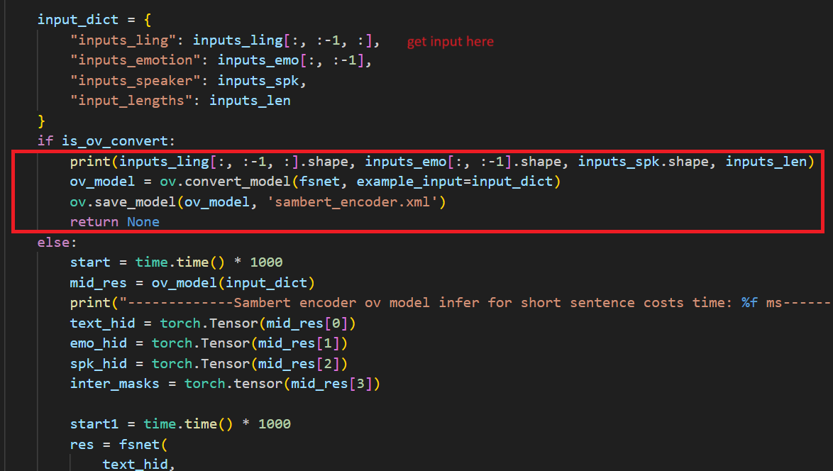
Convert torch modelto openVINO^TM model

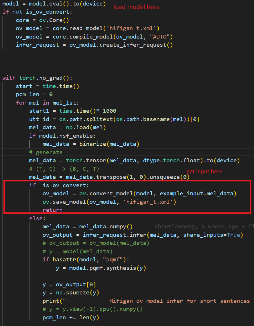
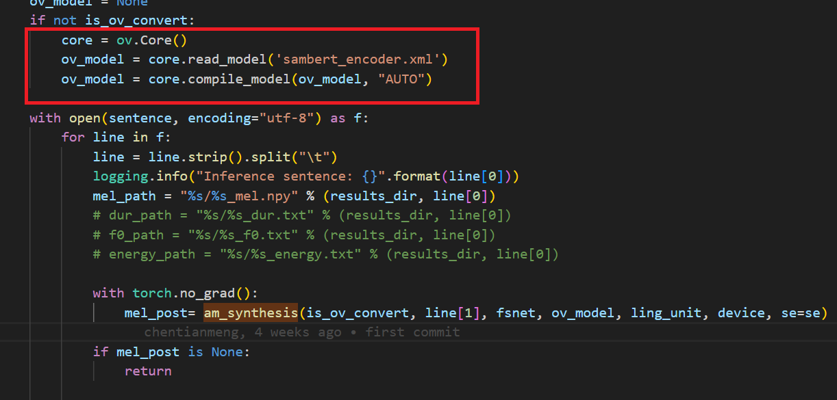
Converting a torch model to OpenVINO^TM requires model inputs. So we usetest.txt as input of SAMBERT and use the res folder as input of HifiGAN.

python kantts/bin/text_to_wav.py --txt test.txt --output_dir res/test_male_ptts_syn --res_zip speech_personal_sambert-hifigan_nsf_tts_zh-cn_pretrain_16k/resource.zip --am_ckpt speech_personal_sambert-hifigan_nsf_tts_zh-cn_pretrain_16k/pretrain_work_dir/tmp_am/ckpt/checkpoint_2400200.pth --voc_ckpt speech_personal_sambert-hifigan_nsf_tts_zh-cn_pretrain_16k/pretrain_work_dir/orig_model/basemodel_16k/hifigan/ckpt/checkpoint_2400000.pth  --se_file speech_personal_sambert-hifigan_nsf_tts_zh-cn_pretrain_16k/pretrain_work_dir/data/se/se.npy --is_ov_convert

Aftera few minutes, you will get two converted OpenVINO^TM model sambert_encoder.xml sambert_encoder.bin and hifigan_t.xml hifigan_t.bin.

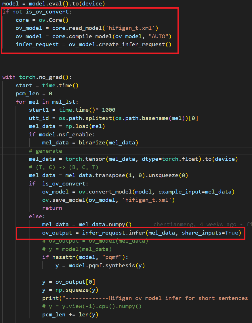
In the code after we load the model and get the inputs, we add the following code to convert the loaded PyTorch backend model to OpenVINO^TM backend model and save it.

Run the inferencewith OpenVINO^TM model

Before running the inference, the res folder should be renamed to allow for comparisons later.

mv res res_pytorch

then run the command below.

python kantts/bin/text_to_wav.py --txt test.txt --output_dir res/test_male_ptts_syn --res_zip speech_personal_sambert-hifigan_nsf_tts_zh-cn_pretrain_16k/resource.zip --am_ckpt speech_personal_sambert-hifigan_nsf_tts_zh-cn_pretrain_16k/pretrain_work_dir/tmp_am/ckpt/checkpoint_2400200.pth --voc_ckpt speech_personal_sambert-hifigan_nsf_tts_zh-cn_pretrain_16k/pretrain_work_dir/orig_model/basemodel_16k/hifigan/ckpt/checkpoint_2400000.pth  --se_file speech_personal_sambert-hifigan_nsf_tts_zh-cn_pretrain_16k/pretrain_work_dir/data/se/se.npy

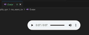
After a few minutes, you will get the wav file in res/test_male_ptts_syn. For example in test.txt we write a random sentence:

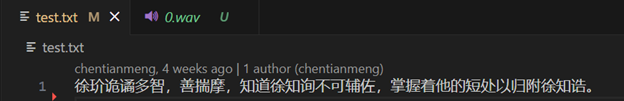
After running pipeline, we will get a 7 seconds wav file under res folder:

In the code we modified the original pytorch banckend inference code so that pipeline uses openvino backend for inference.

Summary

This blog describes about how to run the SAMBERT-HifiGANpipeline using the OpenVINOTM Python API, please see the source code formore details and modifications.

‍

Authors: Fiona Zhao, Xiake Sun, Wenyi Zou, Su Yang, Tianmeng Chen

Model Server reference implementation based on OpenVINO GenAI Package for Edge/Client AI PC Use Case.

openvino.genai/samples/cpp/rag_sample at openvino_genai_serving · sammysun0711/openvino.genai (github.com)

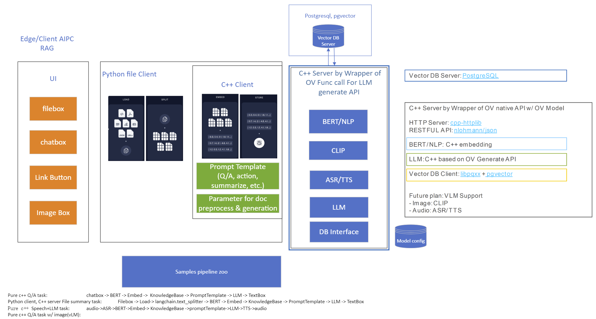
Use Case 1: C++ RAG Sample that supports most popular models like LLaMA 2

This example showcases for Retrieval-Augmented Generation based on text-generation Large Language Models (LLMs): chatglm, LLaMA, Qwen and other models with the same signature and Bert model for embedding feature extraction. The sample fearures ov::genai::LLMPipeline and configures it for the chat scenario. There is also a Jupyter notebook which provides an example of LLM-powered RAG in Python.

Download and convert the model and tokenizers

The --upgrade-strategy eager option is needed to ensure optimum-intel is upgraded to the latest version.

python3 -m pip install --upgrade-strategy eager -r ../../requirements.txt
optimum-cli export openvino --trust-remote-code --model TinyLlama/TinyLlama-1.1B-Chat-v1.0 TinyLlama-1.1B-Chat-v1.0

Setup of PostgreSQL, Libpqxx and Pgvector

Langchain's document Loader and Spliter

1. Load: document_loaders is used to load document data.
2. Split: text_splitter breaks large Documents into smaller chunks. This is useful both for indexing data and for passing it in to a model, since large chunks are harder to search over and won’t in a model’s finite context window.

PostgreSQL

Download postgresql from enterprisedb.(postgresql-16.2-1-windows-x64.exe is tested)

Install PostgreSQL with postgresqltutorial.
Setup of PostgreSQL:
1. Open pgAdmin 4 from Windows Search Bar.
2. Click Browser (left side) > Servers > Postgre SQL 10.
3. Create the user postgres with password openvino (or your own setting)
4. Open SQL Shell from Windows Search Bar to check this setup. 'Enter' to set Server, Database, Port, Username as default and type Password.

Server [localhost]: 
Database [postgres]:
Port [5432]:
Username [postgres]:
Password for user postgres:

libpqxx

'Official' C++ client library (language binding), built on top of C library

Update the source code from https://github.com/jtv/libpqxx in deps\libpqxx

The pipeline connects with DB based on Libpqxx.

pgvector

Open-source vector similarity search for Postgres.

By default, pgvector performs exact nearest neighbor search, which provides perfect recall. It also supports approximate nearest neighbor search (HNSW), which trades some recall for speed.

For Windows, Ensure C++ support in Visual Studio 2022 is installed, then use nmake to build in Command Prompt for VS 2022(run as Administrator). Please follow with the pgvector

Enable the extension (do this once in each database where you want to use it), run SQL Shell from Windows Search Bar with "CREATE EXTENSION vector;".

Printing CREATE EXTENSION shows successful setup of Pgvector.

pgvector-cpp

pgvector support for C++ (supports libpqxx). The headers (pqxx.hpp, vector.hpp, halfvec.hpp) are copied into the local folder rag_sample\include. Our pipeline does the vector similarity search for the chunks embeddings in PostgreSQL, based on pgvector-cpp.

‍

Install OpenVINO, VS2022 and Build this pipeline

Download 2024.2 release from OpenVINO™ archives*. This OV built package is for C++ OpenVINO pipeline, no need to build the source code. Install latest Visual Studio 2022 Community for the C++ dependencies and LLM C++ pipeline editing.

Extract the zip file in any location and set the environment variables with dragging this setupvars.bat in the terminal Command Prompt. setupvars.ps1 is used for terminal PowerShell. <INSTALL_DIR> below refers to the extraction location. Run the following CMD in the terminal Command Prompt.

git submodule update --init
<INSTALL_DIR>\setupvars.bat
cd openvino.genai
cmake -S .\ -B .\build\ && cmake --build .\build\ --config Release -j8
cd .\build\samples\cpp\rag_sample\Release

Notice:

• Install on Windows: Copy all the DLL files of PostgreSQL, OpenVINO and tbb and openvino-genai into the release folder. The SQL DLL files locate in the installed PostgreSQL path like "C:\Program Files\PostgreSQL\16\bin".
• If cmake not installed in the terminal Command Prompt, please use the terminal Developer Command Prompt for VS 2022 instead.
• The openvino tokenizer in the third party needs several minutes to build. Set 8 for -j option to specify the number of parallel jobs.
• Once the cmake finishes, check rag_sample_client.exe and rag_sample_server.exe in the relative path .\build\samples\cpp\rag_sample\Release.
• If Cmake completed without errors, but not find exe, please open the .\build\OpenVINOGenAI.sln in VS2022, and set the solution configuration as Release instead of Debug, then build the llm project within VS2022 again.

Run

Launch RAG Server

rag_sample_server.exe --llm_model_path TinyLlama-1.1B-Chat-v1.0 --llm_device CPU --embedding_model_path bge-large-zh-v1.5 --embedding_device CPU  --db_connection "user=postgres host=localhost password=openvino port=5432 dbname=postgres"

Lanuch RAG Client

rag_sample_client.exe

Lanuch python Client

Use python client to send the message of DB init and send the document chunks to DB for embedding and storing.

python client_get_chunks_embeddings.py --docs test_document_README.md

‍

In the ever-evolving landscape of biopharmaceutical technology and drug development, a recent effort in the field of Cell Analytics for Monoclonal Antibody Production has shed light on the crucial role of Edge AI Technology in navigating complex challenges of scaling and producing solutions.  

In this 2-part blog series, we will explore the use of Intel Edge AI Technology in biopharma and drug development, addressing challenges and providing insights into the development of AI pipelines for cell segmentation and analysis.

Intel has been involved in this process with a variety of partners. One of Intel’s contributions to the cell image project centers around processing brightfield¹ images using an AI pipeline containing multiple deep learning models. The pipeline's purpose is to identify cells and other biological components and provide feedback on dynamic biological characteristics such as cell morphology, viability, and phenotypic changes, among others. Throughout this process, working on cell-AI projects usually brings a unique set of challenges to the forefront.  

First, it is an interdisciplinary field and the knowledge gap between data scientists and biopharma experts requires more back-and-forth clear communications for planning and validity checks. Frequently when attempting to implement AI solutions in the laboratory, data scientists and bench scientists struggle to fully grasp the nature and needs of each other’s role. This lack of mutual understanding can also hinder the usability and scalability of an AI solution needing to be integrated into diverse lab environments.

The second challenge is instrument variability. Different plate reader² microscopes have different hardware, optics, and apertures which cause their produced images not to be consistent. This adds an extra layer of work to assess and address these inconsistencies along the way (like regular tracked calibration and adjustment). Additionally, equipment vendor-to-vendor differences, culture temperature, medium conditions, and genetic modifications can all affect the variability of data and the inherent transferability of the deep learning pipeline. This would drive the need to monitor the performance of DL models at the edge and cloud ML ops components.    

The third challenge is obtaining peer-review labels because the process is based on supervised Machine Learning and obtaining clean accurate labels is very costly and time-consuming.  

And the last challenge is about the model deployment. In most cases, cloud deployment is not an option due to data size and data privacy. Produced images from plate reader microscopes are huge and transferring data to the cloud and sending the results back would create high latency because a huge amount of data must be streamed (30Gb per hour). And more importantly, laboratories are usually not willing to share the data. Due to these two constraints, cloud deployments are not usually an option, and the pipeline must be deployed at the edge.  

Now, let’s talk about a specific application of this technology: the CHO Cell Segmentation Use Case.

CHO Cell Segmentation Use Case

CHO cells, or Chinese Hamster Ovary cells, are a cornerstone in the production of complex protein molecules such as monoclonal antibodies, fusion proteins, hormones, and coagulation factors. Unlike stem cells or CAR-T cells, where the cells themselves are the therapeutic product, in CHO cells, it is the proteins they produce that are of paramount importance. Monitoring the health, viability, and production capability of these cells is a critical step in commercial protein production.

Traditionally, assessing the condition of CHO cells involves a multi-step process that is not only time-consuming but also requires the use of expensive reagents and chemicals. Depending on the process, the workflow can be something like below.  

1. Culture cells  

2. Fix cells – wash in expensive reagents to remove the culture medium.  

3. Permeabilization – wash in more expensive chemicals to permeabilize the cell membrane (to stain for intercellular proteins).

4. Blocking – incubate cells in another expensive reagent to prevent binding of no specific antibodies.

5. Primary Antibody Incubation – antibody specifically to bind to a protein that is being produced.

6. Washing – removing unbound Primary Antibodies using more expensive chemicals.

7. Nuclear staining – use nuclear stain like DAPI to visualize cell nuclei then wash with the same chemicals from the washing step

8. Mounting – get ready to read in the microscope (plate reader¹)

9. Imaging – Stained cells …. count them up and determine the state in the protein production cycle and relative cell health (eventually they peter out and stop producing and the batch needs to be flushed. (Cell count, viability number, etc. are the output not the image)

From culturing to imaging, each step plays a vital role in ensuring the quality of the protein product. However, with the advent of AI and deep learning, there is an opportunity to streamline this workflow significantly. Using an AI pipeline including multiple Deep Learning models and data pre and post-processing, we can go from Step 1 directly to Step 9, removing the majority of the labor and latency in getting actionable results out of a staining workflow and bypassing expensive specialty chemicals requirement. Intel has put together a reference implementation for deploying said pipeline and inferencing of these images on the edge as part of the Cell Image project https://www.cellimage.ie/. OpenVINO Toolkit, OpenVINO Model Server, and AI Connect for Scientific Data are used in this design. Let’s briefly talk about each of these wonderful SW packages in part 2 of this article series. Stay tuned!

Conclusion

In conclusion, the integration of Intel Edge AI Technology into the biopharmaceutical sector represents a transformative step towards more efficient and scalable drug development processes. As we have seen in this first installment of our blog series, the deployment of AI pipelines for cell segmentation and analysis in monoclonal antibody production is not without its challenges. These include bridging the interdisciplinary knowledge gap, managing instrument variability, acquiring peer-reviewed labels, and overcoming the hurdles associated with model deployment.

Despite these challenges, the potential benefits of Edge AI in biopharma are substantial. By leveraging Intel's advanced AI technologies, we can significantly reduce the time and cost associated with traditional cell analysis methods, while also enhancing the accuracy and reliability of the results. The use of edge computing addresses the concerns of data size and privacy, allowing for real-time processing and analysis without the need for cloud transfer.

As we move forward in this blog series, we will delve deeper into the specifics of Intel's Edge AI solutions, including the OpenVINO toolkit, OpenVINO Model Server, and AI Connect for Scientific Data. We will explore how these tools are being applied in real-world scenarios to drive innovation and improve outcomes in the realm of biopharma and drug development in the next part of this series.

Reach out to Intel's Health and Life Sciences team at health.lifesciences@intel.com or learn more about what we do at https://www.intel.com/health.

We'd like to hear from you! Let us know in the comments or discuss – which AI use cases in health and life sciences do you think will have the greatest impact on global health?

If you enjoyed hearing from the Health and Life Sciences team and want to hear more, give this post a like and ensure you subscribe to get the latest updates from the team. 

About the Author

Nooshin Nabizadeh has Ph.D. in Electrical and Computer Engineering from the University of Miami and works at Intel Corporation as AI Solutions Architect. She enjoys photography, writing poetry, reading about psychology and philosophy, and optimizing solutions to run as fast as possible on a given piece of hardware. Connect with her on LinkedIn https://www.linkedin.com/in/nooshin-nabizadeh/ by mentioning this blog.

1. Brightfield microscopy is a widely used technique for observing the morphology of cells and tissues.

2. A plate reader is a laboratory instrument used to obtain images from samples in microtiter plates. The reader shines a specific calibrated frequency of light (UV, visible, fluorescence, etc.) through the samples in the wells of the plate. Plate reader microscopy data sets have inherent variability which drives the requirement of regular tracked calibration and adjustment.

‍

Authors: Nikita Savelyev, Alexander Kozlov, Ekaterina Aidova, Maxim Proshin

‍

Introduction

Whisper is a general-purpose speech recognition model from OpenAI. The model can transcribe speech across dozens of languages and even handle poor audio quality or excessive background noise. You can find more information about this model in the research paper, OpenAI blog, model card and GitHub repository.

Recently, a distilled variant of the model called Distil-Whisper has been proposed in the paper Robust Knowledge Distillation via Large-Scale Pseudo Labelling. Compared to Whisper, Distil-Whisper runs several times faster with 50% fewer parameters, while performing to within 1% word error rate (WER) on out-of-distribution evaluation data.

Whisper is a Transformer-based encoder-decoder model, also referred to as a sequence-to-sequence model. It maps a sequence of audio spectrogram features to a sequence of text tokens. First, the raw audio inputs are converted to a log-Mel spectrogram by action of the feature extractor. Then, the Transformer encoder encodes the spectrogram to form a sequence of encoder hidden states. Finally, the decoder autoregressively predicts text tokens, conditional on both the previous tokens and the encoder's hidden states.

You can see the model architecture in the diagram below:

In this article, we would like to demonstrate how to improve Whisper and Distil-Whisper inference speed with OpenVINO for Intel hardware. Additionally, we show how to make models even faster by applying 8-bit Post-training Quantization with Neural Network Compression Framework (NNCF). In the end we present evaluation results from accuracy and performance standpoints on a large-scale dataset.

All code snippets presented in this article are from the Automatic speech recognition using Distil-Whisper and OpenVINO Jupyter notebook, so you can follow along.

‍

Converting Model to OpenVINO format

We are going to load models from Hugging Face Hub with the help of Optimum Intel library which makes it easier to load and run OpenVINO-optimized models. For more details, pleaes refer to the Hugging Face Optimum documentation.

For example, the following code loads the Distil-Whisper large-v2 model ready for inference with OpenVINO.

from optimum.intel.openvino import OVModelForSpeechSeq2Seq

model_id = "distil-whisper/distil-large-v2"
model_path = Path(model_id)
if not model_path.exists():
    ov_model = OVModelForSpeechSeq2Seq.from_pretrained(
        model_id, export=True, compile=False, load_in_8bit=False)
    ov_model.half()
    ov_model.save_pretrained(model_path)
else:
    ov_model = OVModelForSpeechSeq2Seq.from_pretrained(
        model_path, compile=False)

Models from the Distil-Whisper family are available at Distil-Whisper Models collection and Whisper models are available at OpenAI Hugging Face page.

To transcribe an input audio with the loaded model, we first compile the model to the device of choice and then call generate() method on input features prepared by corresponding processor.

from transformers import AutoProcessor

processor = AutoProcessor.from_pretrained(model_id)

ov_model.to("AUTO")
ov_model.compile()

# ... load input audio and reference text
input_features = processor(input_audio).input_features
predicted_ids = ov_model.generate(input_features)
transcription = processor.batch_decode(predicted_ids, skip_special_tokens=True)[0]
print(f"Reference: {reference_text}")
print(f"Result: {transcription}")

The output is the following. As you can see the transcription equals the reference text.

Reference: MISTER QUILTER IS THE APOSTLE OF THE MIDDLE CLASSES AND WE ARE GLAD TO WELCOME HIS GOSPEL
Result:  Mr. Quilter is the apostle of the middle classes, and we are glad to welcome his gospel.

‍

Running Post-Training Quantization with NNCF

NNCF enables post-training quantization by adding quantization layers into the model graph and then using a subset of the training dataset to initialize parameters of these additional quantization layers. During quantization, some layers (e.g., MatMuls, Convolutions) are transformed to be executed in INT8 instead of FP16/FP32. If a quantized operation is parameterized then its corresponding weight variable is also converted to INT8.

In general, the optimization process contains the following steps:

1. Create a calibration dataset for quantization.
2. Run nncf.quantize() to obtain quantized encoder and decoder models.
3. Serialize the INT8 models using openvino.save_model() function.

‍

Whisper model consists of an encoder and decoder submodels. Furthermore, for the decoder model its forward() signature is different for the first call compared to all subsequent calls. During the first call, key-value cache is empty and is not needed for decoder inference. Starting from the second call, key-value cache is fed to the decoder. Because of this, these two cases are represented by two separate OpenVINO models: openvino_decoder_model.xml and openvino_decoder_with_past_model.xml. Since the first decoder model is inferred only once it does not make much sense to quantize it. So, we apply quantization to the encoder and the decoder with past models.

The first step towards quantization is collecting calibration data. For that, we need to collect some number of model inputs for both models. To do that, we patch OpenVINO model request objects with an InferRequestWrapper class instance that will intercept model inputs during inference and store them in a list. We infer the model on about 50 samples from validation split of librispeech_asr dataset.

def collect_calibration_dataset(ov_model: OVModelForSpeechSeq2Seq, calibration_dataset_size: int):
    # Overwrite model request properties, saving the original ones for restoring later
    original_encoder_request = ov_model.encoder.request
    original_decoder_with_past_request = ov_model.decoder_with_past.request
    encoder_calibration_data = []
    decoder_calibration_data = []
    ov_model.encoder.request = InferRequestWrapper(original_encoder_request, encoder_calibration_data)
    ov_model.decoder_with_past.request = InferRequestWrapper(original_decoder_with_past_request,
                                                             decoder_calibration_data)

    calibration_dataset = load_dataset("librispeech_asr", "clean", split="validation", streaming=True)
    for sample in islice(calibration_dataset, calibration_dataset_size):
        input_features = extract_input_features(sample)
        ov_model.generate(input_features)

    ov_model.encoder.request = original_encoder_request
    ov_model.decoder_with_past.request = original_decoder_with_past_request

    return encoder_calibration_data, decoder_calibration_data

With the collected calibration data for encoder and decoder models we can proceed to quantization itself. Let's examine the quantization call for the encoder model. For the decoder model, it is similar.

quantized_encoder = nncf.quantize(
    ov_model.encoder.model,                     # ov.Model object of the encoder model
    nncf.Dataset(encoder_calibration_data),     # calibration data wrapped in a nncf.Dataset object
    subset_size=len(encoder_calibration_data),  # number of samples to calibrate on (all are chosen)
    model_type=nncf.ModelType.TRANSFORMER,      # providing the information that Whisper encoder is of
    # a Transformer architecture
    advanced_parameters=nncf.AdvancedQuantizationParameters(smooth_quant_alpha=0.50)    # Smooth Quant 
    # algorithm reduces activation quantization error; optimal alpha was obtained through grid search
)
ov.save_model(quantized_encoder, quantized_model_path / "openvino_encoder_model.xml")

After both models are quantized and saved, the quantized Whisper model can be loaded and run the same way as shown previously. Comparing the transcriptions produced by original and quantized models results in the following.

Original :  Mr. Quilter is the apostle of the middle classes, and we are glad to welcome his gospel.
Quantized:  Mr. Quilter is the apostle of the middle classes, and we are glad to welcome his gospel.

As you can see for the quantized distil-whisper-large-v2 transcription is the same.

‍

Evaluating on Common Voice Dataset

We evaluate Whisper and Distil-Whisper large-v2 model variants on a Common Voice 13.0 speech-to-text dataset. We use en/test split containing 16372 audio samples amounting to about 27 hours of recordings.

The evaluation is done across three model types: original PyTorch model, original OpenVINO model and quantized OpenVINO model. Additionally, we run tests on three Intel CPUs: Cascade Lake Intel(R) Core(TM) i9-10980XE, Ice Lake Intel(R) Xeon(R) Gold 6338 and Sapphire Rapids Intel(R) Xeon(R) Gold 6430L.

For all combinations above we measure transcription time and accuracy. When measuring time for a model we sum up generate() call durations for all audio samples. Transcription accuracy is represented as Accuracy = (100 - WER), WER stands for Word Error Rate. We compute accuracy for each audio sample and then take the average value across the dataset. The results are given in the table below.

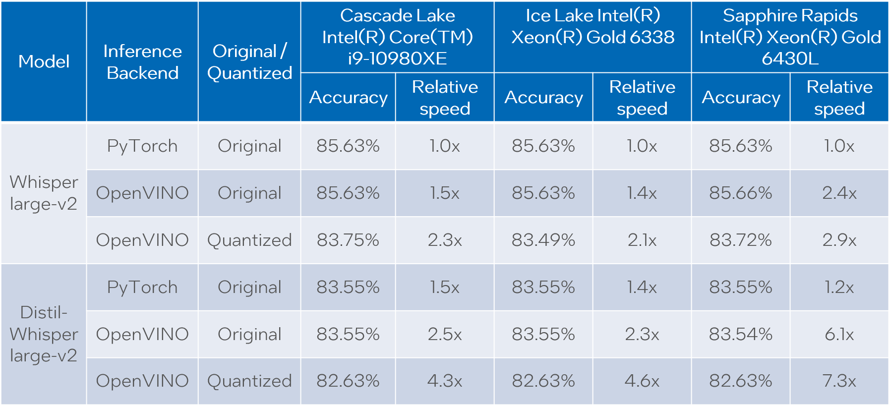
Please note that we report transcription time in relative terms such that the values for each CPU are normalized over its corresponding column. The duration of audio data in the dataset is 27.06 hours and the absolute transcription time values for Whisper large-v2 PyTorch on each CPU are:

• 20.35 hours for Core i9-10980XE
• 14.09 hours for Xeon Gold 6338
• 15.03 hours for Xeon Gold 6430L

‍

Based on the results we can conclude that:

1. OpenVINO models execute 1.4x - 5.1x faster than PyTorch models with pretty much the same accuracy across all cases.
2. When compared to original PyTorch models, quantized OpenVINO models provide 2.1x - 6.1x performance boost with 1-2% accuracy drop.

‍

NOTE: in terms of this article we focus on presenting performance values. Accuracy of quantized models can be improved with a more careful selection of calibration data.

Notices and Disclaimers:

Performance varies by use, configuration, and other factors. Learn more at www.intel.com/PerformanceIndex. Performance results are based on testing as of dates shown in configurations and may not reflect all publicly available updates. No product or component can be absolutely secure. Intel technologies may require enabled hardware, software or service activation.

The products described may contain design defects or errors known as errata which may cause the product to deviate from published specifications. Current characterized errata are available on request.

Test Configuration: Intel® Core™ i9-10980XE CPU Processor at 3.00GHz with DDR4 128 GB at 3000MHz, OS: Ubuntu 20.04.3 LTS; Intel® Xeon® Gold 6338 CPU Processor at 2.00GHz with DDR4 256 GB at 3200MHz, OS: Ubuntu 20.04.3 LTS; Intel® Xeon® Gold 6430L CPU Processor at 1.90GHz with DDR5 1024 GB at 4800MHz, OS: Ubuntu 20.04.6 LTS. Testing was performed using distil-whisper-asr notebook for model export and whisper evaluation notebook for model evaluation.

The test was conducted by Intel in December 2023.

‍

Conclusion

We demonstrated how to load and run Whisper and Distil-Whisper models for audio transcription task with OpenVINO and Optimum Intel, and how to perform INT8 post-training quantization of these models with NNCF. Further we evaluated these models on a large scale speech-to-text dataset across multiple CPU devices. The evaluation results show a significant performance boost of OpenVINO vs PyTorch models without loss of transcription quality, and even a larger boost with a tolerable accuracy drop when we apply INT8 quantization.

‍

‍

Introduction

Latent Consistency Models (LCMs) is the next generation of generative models after Latent Diffusion Models (LDMs). While Latent Diffusion Models (LDMs) like Stable Diffusion are capable of achieving the outstanding quality of generation, they often suffer from the slowness of the iterative image denoising process. LCM is an optimized version of LDM. Inspired by Consistency Models (CM), Latent Consistency Models (LCMs) enabled swift inference with minimal steps on any pre-trained LDMs, including Stable Diffusion. The Consistency Models is a new family of generative models that enables one-step or few-step generation. More details about the proposed approach and models can be found using the following resources: project page, paper, original repository.

This article will demonstrate a C++ application of the LCM model with Intel’s OpenVINO™ C++ API on Linux systems. For model inference performance and accuracy, the C++ pipeline is well aligned with the Python implementation.

The full implementation of the LCM C++ demo described in this post is available on the GitHub: openvino.genai/lcm_dreamshaper_v7.

Model Conversion

To leverage efficient inference with OpenVINO™ runtime on Intel platforms, the original model should be converted to OpenVINO™ Intermediate Representation (IR).

LCM model

Optimum Intel can be used to load SimianLuo/LCM_Dreamshaper_v7 model from Hugging Face Hub and convert PyTorch checkpoint to the OpenVINO™ IR on-the-fly, by setting export=True when loading the model, like:

from optimum.intel.openvino import OVLatentConsistencyModelPipeline

model = OVLatentConsistencyModelPipeline.from_pretrained("SimianLuo/LCM_Dreamshaper_v7", export=True)
model.save_pretrained("ov_lcm_model")

Tokenizer

OpenVINO Tokenizers is an extension that adds text processing operations to OpenVINO Inference Engine. In addition, the OpenVINO Tokenizers project has a tool to convert a HuggingFace tokenizer into OpenVINO IR model tokenizer and detokenizer: it provides the convert_tokenizer function that accepts a tokenizer Python object and returns an OpenVINO Model object:

from transformers import AutoTokenizer
from openvino_tokenizers import convert_tokenizer
from openvino import compile_model, save_model

hf_tokenizer = AutoTokenizer.from_pretrained(tokenizer_path)
ov_tokenizer_encoder = convert_tokenizer(hf_tokenizer)
save_model(ov_tokenizer_encoder, "ov_tokenizer.xml")

Note: Currently OpenVINO Tokenizers can be inferred on CPU devices only.

Conversion step

You can find the full script for model conversion at the original repo.

Note: The tutorial assumes that the current working directory is and <openvino.genai repo>/image_generation/lcm_ dreamshaper_v7/cpp all paths are relative to this folder.

Let’s prepare a Python environment and install dependencies:

conda create -n openvino_lcm_cpp python==3.10
conda activate openvino_lcm_cpp
conda install -c conda-forge 'openvino>=2023.3.0'
python -m pip install -r scripts/requirements.txt
python -m pip install ../../../thirdparty/openvino_contrib/modules/custom_operations/[transformers]

Now we can use the script scripts/convert_model.py to download and convert models:

cd scripts
python convert_model.py -lcm "SimianLuo/LCM_Dreamshaper_v7" -t FP16

C++ Pipeline

Pipeline flow

Let’s now talk about the logical structure of the LCM model pipeline.

Just like the classic Stable Diffusion pipeline, the LCM pipeline consists of three important parts:
- A text encoder to create a condition to generate an image from a text prompt.
- U-Net for step-by-step denoising the latent image representation.
- Autoencoder (VAE) for decoding the latent space to an image.

The pipeline takes a latent image representation and a text prompt transformed to text embedding via CLIP’s text encoder as an input. The initial latent image representation is generated using random noise generator. LCM uses a guidance scale for getting time step conditional embeddings as input for the diffusion process, while in Stable Diffusion, it used for scaling output latents.

Next, the U-Net iteratively denoises the random latent image representations while being conditioned on the text embeddings. The output of the U-Net, being the noise residual, is used to compute a denoised latent image representation via a scheduler algorithm. LCM introduces its own scheduling algorithm that extends the denoising procedure introduced by denoising diffusion probabilistic models (DDPMs) with non-Markovian guidance. The denoising process is repeated for a given number of times to step-by-step retrieve better latent image representations. When complete, the latent image representation is decoded by the decoder part of the variational auto encoder.

The C++ implementations of the scheduler algorithm and LCM pipeline are available at the following links: LCM Scheduler, LCM Pipeline.

LoRA support

LoRA (Low-Rank Adaptation) is a training technique for fine-tuning Stable Diffusion models. There are various LoRA models available on https://civitai.com/tag/lora.

The main idea for LoRA weights enabling, is to append weights onto the OpenVINO LCM models at runtime before compiling the Unet/text_encoder model. The method is to extract LoRA weights from safetensors file, find the corresponding weights in Unet/text_encoder model and insert the LoRA bias weights. The common approach to add LoRA weights looks like:

The original LoRA safetensor model is loaded via safetensors.h. The layer name and weight of LoRA are modified with Eigen Lib and inserted into Unet/text_encoder OpenVINO model using ov::pass::MatcherPass - you can see the implementation in the file common/diffusers/src/lora.cpp.

To run the LCM demo with the LoRA model, first download LoRA, for example: LoRa/Soulcard.

Build and Run LCM demo

Let’s start with the dependencies installation:‍

conda activate openvino_lcm_cpp
conda install -c conda-forge eigen c-compiler cxx-compiler make

Now we can build the application:

cmake -DCMAKE_BUILD_TYPE=Release -S . -B build
cmake --build build --config Release --parallel
cd build

‍‍And finally we’re ready to run the LCM demo. By default the positive prompt is set to: “a beautiful pink unicorn”.

Please note, that the quality of the resulting image depends on the quality of the random noise generator, so there is a difference for output images generated by the C++ noise generator and the PyTorch generator. Use oprion -r to read the PyTorch generated noise from the provided textfiles for the alignment with Python pipeline.
‍

Note: Run ./lcm_dreamshaper -h to see all the available demo options

Let’s try to run the application in a few modes:

Read the numpy latent input and noise for scheduler instead of C++ std lib for the alignment with Python pipeline: ./lcm_dreamshaper -r‍

Generate image with C++ std lib generated latent and noise : ./lcm_dreamshaper

‍

‍

Generate image with Soulcard LoRa and C++ generated latent and noise: ./lcm_dreamshaper -r -l path/to/soulcard.safetensors

‍

See Also

1. Optimizing Latent Consistency Model for Image Generation with OpenVINO™ and NNCF
2. Image generation with Latent Consistency Model and OpenVINO
3. C++ Pipeline for Stable Diffusion v1.5 with Pybind for Lora Enabling
4. Enable LoRA weights with Stable Diffusion Controlnet Pipeline

‍

Authors: Fiona Zhao, Xiake Sun, Su Yang

The purpose is to demonstrate the use of C++ native OpenVINO API.

For model inference performance and accuracy, the pipelines of C++ and python are well aligned.

Source code github: OV_SD_CPP.

Step 1: Prepare Environment

Setup in Linux:

C++ pipeline loads the Lora safetensors via Pybind

conda create -n SD-CPP python==3.10
conda activate SD-CPP
conda install numpy safetensors pybind11 

C++ Dependencies:

• OpenVINO: Tested with OpenVINO 2023.1.0.dev20230811 pre-release
• Boost: Install with sudo apt-get install libboost-all-dev for LMSDiscreteScheduler's integration
• OpenCV: Install with sudo apt install libopencv-dev for image saving

Notice:

SD Preparation in two steps above could be auto implemented with build_dependencies.sh in the scripts directory.

cd scripts
chmod +x build_dependencies.sh
./build_dependencies.sh

Step 2: Prepare SD model and Tokenizer Model

• SD v1.5 model:

Refer this link to generate SD v1.5 model, reshape to (1,3,512,512) for best performance.

With downloaded models, the model conversion from PyTorch model to OpenVINO IR could be done with script convert_model.py in the scripts directory.

python -m convert_model.py -b 1 -t <INT8|FP16|FP32> -sd Path_to_your_SD_model

Lora enabling with safetensors, refer this blog.

SD model dreamlike-anime-1.0 and Lora soulcard are tested in this pipeline.

• Tokenizer model:

1. The script convert_sd_tokenizer.py in the scripts dir could serialize the tokenizer model IR
2. Build OpenVINO extension:

git clone https://github.com/apaniukov/openvino_contrib/  -b tokenizer-fix-decode

Refer to PR OpenVINO custom extension ( new feature still in experiments )

3. read model with extension in the SD pipeline

Step 3: Build Pipeline

source /Path_to_your_OpenVINO_package/setupvars.sh
conda activate SD-CPP
mkdir build && cd build
cmake -DCMAKE_BUILD_TYPE=Release ..
make

Step 4: Run Pipeline

./SD-generate -p <posPromp> -n <negPrompt> -d <device> -s <seed> --height <output image> --width <output image> --log <use logger> -c <use cache> -e <useOVExtension> -r <readNPLatent> -m <modelPath> -t <type of model IR> -l <lora.safetensors> -a <alpha> -h <help>

Usage: OV_SD_CPP [OPTION...]

• -p, --posPrompt arg Initial positive prompt for SD (default: cyberpunk cityscape like Tokyo New York with tall buildings at dusk golden hour cinematic lighting)
• -n, --negPrompt arg Default negative prompt is empty with space (default: )
• -d, --device arg AUTO, CPU, or GPU (default: CPU)
• -s, --seed arg Number of random seed to generate latent (default: 42)
• --height arg height of output image (default: 512)
• --width arg width of output image (default: 512)‍
• --log arg Generate logging into log.txt for debug
• -c, --useCache Use model caching
• -e, --useOVExtension Use OpenVINO extension for tokenizer‍
• -r, --readNPLatent Read numpy generated latents from file‍
• -m, --modelPath arg Specify path of SD model IR (default: /YOUR_PATH/SD_ctrlnet/dreamlike-anime-1.0)‍
• -t, --type arg Specify precision of SD model IR (default: FP16_static)‍
• -l, --loraPath arg Specify path of lora file. (*.safetensors). (default: /YOUR_PATH/soulcard.safetensors)‍
• -a, --alpha arg alpha for lora (default: 0.75)
• -h, --help Print usage

Example:

Positive prompt: cyberpunk cityscape like Tokyo New York with tall buildings at dusk golden hour cinematic lighting.

Negative prompt: (empty, here couldn't use OV tokenizer, check the issues for details).

Read the numpy latent instead of C++ std lib for the alignment with Python pipeline.

• Generate image without lora

./SD-generate -r -l ""

• Generate image with Soulcard Lora

./SD-generate -r

• Generate the debug logging into log.txt

./SD-generate --log

Benchmark:

The performance and image quality of C++ pipeline are aligned with Python.

To align the performance with Python SD pipeline, C++ pipeline will print the duration of each model inferencing only.

For the diffusion part, the duration is for all the steps of Unet inferencing, which is the bottleneck.

For the generation quality, be careful with the negative prompt and random latent generation.

Limitation:

• Pipeline features:

- Batch size 1
- LMS Discrete Scheduler
- Text to image

• Program optimization: now parallel optimization with std::for_each only and add_compile_options(-O3 -march=native -Wall) with CMake
• The pipeline with INT8 model IR not improve the performance
• Lora enabling only for FP16

• Random generation fails to align, C++ random with MT19937 results is differ from numpy.random.randn(). Hence, please use -r, --readNPLatent for the alignment with Python
• OV extension tokenizer cannot recognize the special character, like “.”, ”,”, “”, etc. When write prompt, need to use space to split words, and cannot accept empty negative prompt. So use default tokenizer without config -e, --useOVExtension, when negative prompt is empty

‍

Setup in Windows 10 with VS2019:

1. Python env: Setup Conda env SD-CPP with the anaconda prompt terminal

2. C++ dependencies:

• OpenVINO and OpenCV:

Download and setup Environment Variable: add the path of bin and lib (System Properties -> System Properties -> Environment Variables -> System variables -> Path )

• Boost:

- Download from sourceforge

- Unzip

- Setup: bootstrap.bat

- Build: b2.exe

- Install: b2.exe install

Installed boost in the path C:/Boost, add CMakeList with "SET(BOOST_ROOT"C:/Boost")"

3. Setup of conda env SD-CPP and Setup OpenVINO with setupvars.bat

4. CMake with build.bat like:

rmdir /Q /S build
mkdir build
cd build
cmake -G "Visual Studio 16 2019" -A x64 ^
 -DCMAKE_BUILD_TYPE=Release ^
      ..
cmake --build . --config Release
cd ..

5. Setup of Visual Studio with release and x64, and build: open .sln file in the build Dir

6. Run the SD_generate.exe

‍

Introduction

Stable Diffusion (SD) is a state-of-the-art latent text-to-image diffusion model that generates photorealistic images from text. Recently, many fine-tuning technologies proposed to create custom Stable Diffusion pipelines for personalized image generation, such as Textual Inversion, Low-Rank Adaptation (LoRA). We’ve already published a blog for enabling LoRA with Stable Diffusion + ControlNet pipeline.

In this blog, we will focus on enabling pre-trained textual inversion with Stable Diffusion via Optimum-Intel. The feature is available in the latest Optimum-Intel, and documentation is available here.

Textual Inversion is a technique for capturing novel concepts from a small number of example images in a way that can later be used to control text-to-image pipelines. It does so by learning new “words” in the embedding space of the pipeline’s text encoder.

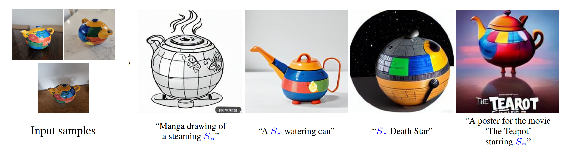
As Figure 1 shows, you can teach new concepts to a model such as Stable Diffusion for personalized image generation using just 3-5 images.

Hugging Face Diffusers and Stable Diffusion Web UI provides useful tools and guides to train and save custom textual inversion embeddings. The pre-trained textual inversion embeddings are widely available in sd-concepts-library and civitai, which can be loaded for inference with the StableDiffusionPipeline using Pytorch as the runtime backend.

Here is an example to load pre-trained textual inversion embedding sd-concepts-library/cat-toy to inference with Pytorch backend.

from diffusers import StableDiffusionPipeline

model_id = "runwayml/stable-diffusion-v1-5"
pipe = StableDiffusionPipeline.from_pretrained(model_id)
pipe.load_textual_inversion("sd-concepts-library/cat-toy")
prompt = "A <cat-toy> backpack"

image = pipe(prompt, num_inference_steps=50).images[0]
image.save("cat-backpack.png")

Optimum-Intel provides the interface between the Hugging Face Transformers and Diffusers libraries to leverage OpenVINO^TM runtime to accelerate end-to-end pipelines on Intel architectures.

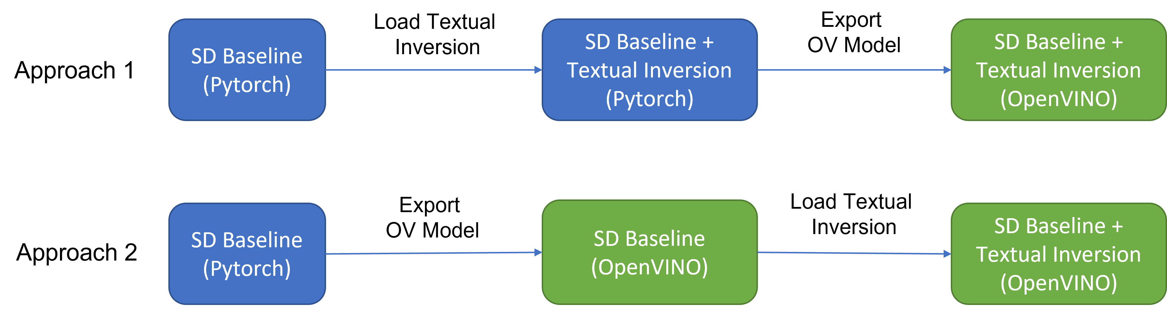
As Figure 2 shows that two approaches are available to enable textual inversion with Stable Diffusion via Optimum-Intel.

Although approach 1 seems quite straightforward and does not need any code modification in Optimum-Intel, the method requires the re-export ONNX model and then model conversion to the OpenVINO^TM IR model whenever the SD baseline model is merged with anew textual inversion.

Instead, we propose approach 2 to support OVStableDiffusionPipelineBase to load pre-trained textual inversion embeddings in runtime to save disk storage while keeping flexibility.

• Save disk storage: We only need to save an SD baseline model converted to OpenVINO^TM IR (e.g.: SD-1.5 ~5GB) and multiple textual embeddings (~10KB-100KB), instead of multiple SD OpenVINO^TM IR with textual inversion embeddings merged (~n *5GB), since disk storage is limited, especially for edge/client use case.
• Flexibility: We can load (multiple) pre-trained textual inversion embeddings in the SD baseline model in runtime quickly, which supports the combination of embeddings and avoid messing up the baseline model.

‍

How to enable textual inversion in runtime?

We implemented OVTextualInversionLoaderMixinbased on diffusers.loaders.TextualInversionLoaderMixin with the following features:

• Load and parse textual embeddings saved as*.bin, *.pt, *.safetensors as a list of Tensors.
• Update tokenizer for new “words” using new token id and expand vocabulary size.
• Update text encoder embeddings via InsertTextEmbedding class based on OpenVINO^TM ngraph transformation.

‍

For the implementation details of OVTextualInversionLoaderMixin, please refer to here. 

Here is the sample code for InsertTextEmbedding class:

class InsertTextEmbedding(MatcherPass):
    r"""
    OpenVINO ngraph transformation for inserting pre-trained texual inversion embedding to text encoder
    """

    def __init__(self, token_ids_and_embeddings):
        MatcherPass.__init__(self)
        self.model_changed = False
        param = WrapType("opset1.Constant")

        def callback(matcher: Matcher) -> bool:
            root = matcher.get_match_root()
            if root.get_friendly_name() == TEXTUAL_INVERSION_EMBEDDING_KEY:
                add_ti = root
                consumers = matcher.get_match_value().get_target_inputs()
                for token_id, embedding in token_ids_and_embeddings:
                    ti_weights = ops.constant(embedding, Type.f32, name=str(token_id))
                    ti_weights_unsqueeze = ops.unsqueeze(ti_weights, axes=0)
                    add_ti = ops.concat(
                        nodes=[add_ti, ti_weights_unsqueeze],
                        axis=0,
                        name=f"{TEXTUAL_INVERSION_EMBEDDING_KEY}.textual_inversion_{token_id}",
                    )

                for consumer in consumers:
                    consumer.replace_source_output(add_ti.output(0))

                # Use new operation for additional matching
                self.register_new_node(add_ti)

            # Root node wasn't replaced or changed
            return False

        self.register_matcher(Matcher(param, "InsertTextEmbedding"), callback)

InsertTextEmbeddingclass utilizes OpenVINO^TM ngraph MatcherPass function to insert subgraph into the model. Please note, the MacherPass function can only filter layers by type, so we run two phases of filtering to find the layer that matched with the pre-defined key in the model:

• Filter all Constant layers to trigger the callback function.
• Filter layer name with pre-defined key “TEXTUAL_INVERSION_EMBEDDING_KEY” in the callback function

‍

If the root name matched the pre-defined key, we will loop all parsed textual inversion embedding and token id pair and create a subgraph (Constant + Unsqueeze + Concat) by OpenVINO^TM operation sets to insert into the text encoder model. In the end, we update the root output node with the last node in the subgraph.

Figure 3 demonstrates the workflow of InsertTextEmbedding OpenVINO^TM ngraph transformation. The left part shows the subgraph in SD 1.5 baseline text encoder model, where text embedding has a Constant node with shape [49408, 768], the 1st dimension is consistent with the original tokenizer (vocab size 49408), and the second dimension is feature length of each text embedding.

When we load (multiple) textual inversion, all textual inversion embeddings will be parsed as a list of tensors with shape[768], and each textual inversion constant will be unsqueezed and concatenated with original text embeddings. The right part is the result of applying InsertTextEmbedding ngraph transformation on the original text encoder, the green rectangle represents merged textual inversion subgraph.

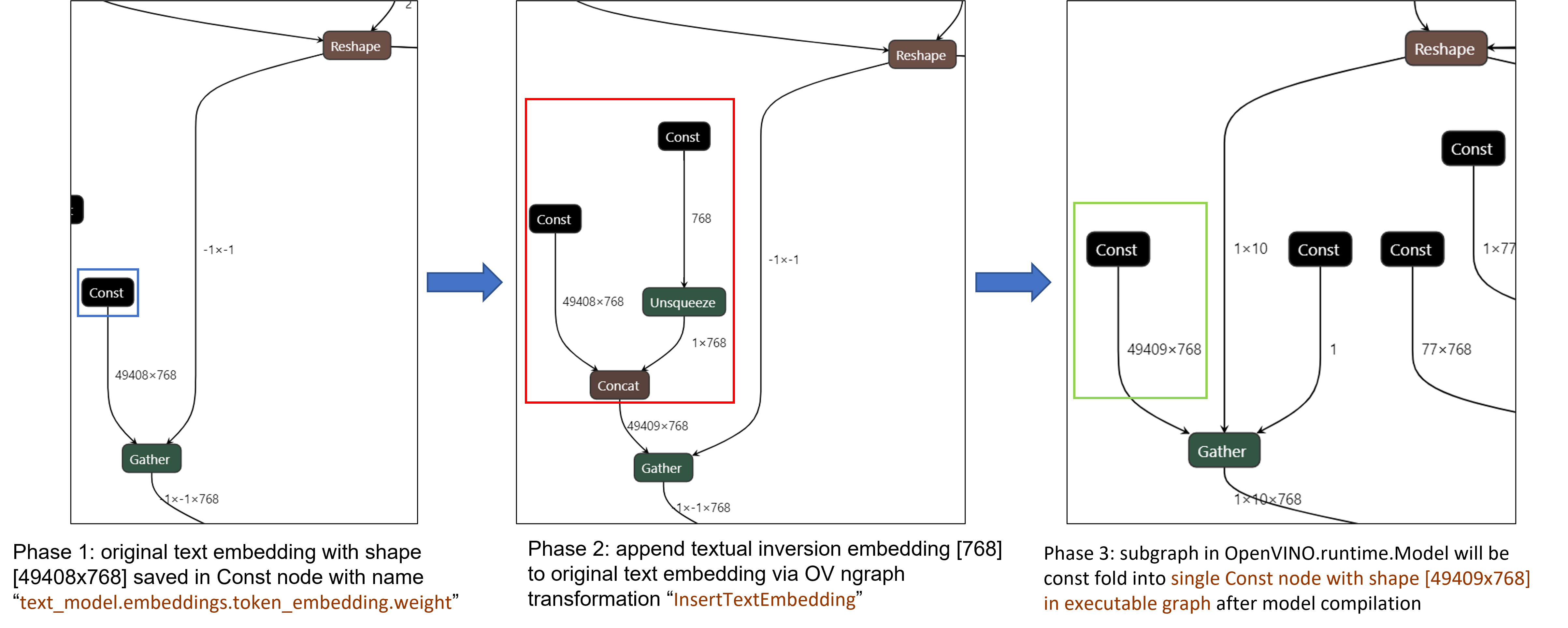
As Figure 4 shows, In the first phase, the original text embedding (marked as blue rectangle) is saved in Const node “text_model.embeddings.token_embedding.weight” with shape [49408,768], after InsertTextEmbedding ngraph transformation, new subgraph (marked as red rectangle) will be created in 2nd phase. In the 3rd phase, during model compilation, the new subgraph will be const folding into a single const node (marked as green rectangle) with a new shape [49409,768] by OpenVINO^TM ConstantFolding transformation.

Stable Diffusion Textual Inversion Sample

Here are textual inversion examples verified with Stable Diffusion v1.5, Stable Diffusion v2.1 and Stable Diffusion XL 1.0 Base pipeline with latest optimum-intel

Setup Environment

conda create -n optimum-intel python=3.10
conda activate optimum-intel
python -m pip install "optimum-intel[openvino]"@git+https://github.com/huggingface/optimum-intel.git
python -m pip install transformers, diffusers, safetensors
python -m pip install invisible-watermark>=0.2.0

Run SD 1.5 + Cat-Toy Textual Inversion Example

from optimum.intel import OVStableDiffusionPipeline
import numpy as np

model_id = "runwayml/stable-diffusion-v1-5"
prompt = "A <cat-toy> back-pack"
np.random.seed(42)

# Run pipeline without textual inversion
pipe = OVStableDiffusionPipeline.from_pretrained(model_id, compile=False)
pipe.compile()
image1 = pipe(prompt, num_inference_steps=50).images[0]
image1.save("sd_v1.5_without_cat_toy_ti.png")

# Run pipeline with textual inversion
pipe.clear_requests()
pipe.load_textual_inversion("sd_concepts/cat-toy", "<cat-toy>")
pipe.compile()
image2 = pipe(prompt, num_inference_steps=50).images[0]
image2.save("sd_v1.5_with_cat_toy_ti.png")

Run SD 2.1 + Midjourney 2.0 Textual Inversion Example

from optimum.intel import OVStableDiffusionPipeline
import numpy as np

model_id = "stabilityai/stable-diffusion-2-1"
prompt = "A <midjourney> style photo of an astronaut riding a horse on mars"
np.random.seed(42)

# Run pipeline without midjourney textual inversion
pipe = OVStableDiffusionPipeline.from_pretrained(model_id, compile=False, cache_dir=None)
pipe.compile()
image1 = pipe(prompt, num_inference_steps=50).images[0]
image1.save("sd_v2.1_without_midjourney_ti.png")

# Run pipeline with midjourney textual inversion
pipe.clear_requests()
pipe.load_textual_inversion("midjourney_sd_2_0", "<midjourney>")
pipe.compile()
image2 = pipe(prompt, num_inference_steps=50).images[0]
image2.save("sd_v2.1_with_midjourney_ti.png")

Run SDXL 1.0 Base + CharTurnerV2 Textual Inversion Example

from optimum.intel import OVStableDiffusionXLPipeline
import numpy as np

model_id = "stabilityai/stable-diffusion-xl-base-1.0"
prompt = "charturnerv2, multiple views of the same character in the same outfit, a character turnaround of a beautiful woman wearing a red jacket and black shirt, best quality, intricate details."
np.random.seed(112)

pipe = OVStableDiffusionXLPipeline.from_pretrained(model_id, export=False, compile=False, cache_dir=None)

# Run pipeline without textual inversion
pipe.compile()
image1 = pipe(prompt, num_inference_steps=50).images[0]
image1.save("sdxl_base_1.0_without_charturnerv2_ti.png")

# Run pipeline with textual inversion
pipe.clear_requests()
pipe.load_textual_inversion("./charturnerv2.pt", "charturnerv2")
pipe.compile()
image2 = pipe(prompt, num_inference_steps=50).images[0]
image2.save("sdxl_base_1.0_with_charturnerv2_ti.png")

Conclusion

In this blog, we proposed to load textual inversion embedding in the stable diffusion pipeline in runtime to save disk storage while keeping flexibility.

• Implemented OVTextualInversionLoaderMixin to update tokenizer with additional token id and update text encoder with InsertTextEmbedding OpenVNO ngraph transformation.
• Provides sample code to load textual inversion with SD 1.5, SD 2.1, and SDXL 1.0 Base and inference with Optimum-Intel

‍

Reference

An Image is Worth One Word: Personalizing Text-to-Image Generation using Textual Inversion

Optimum-Intel Text-to-Image with Textual Inversion

Hugging Face Textual Inversion

Authors: Zhen Zhao(Fiona), Kunda Xu

Low-Rank Adaptation(LoRA) is a novel technique introduced to deal with the problem of fine-tuning Diffusers and Large Language Models (LLMs). In the case of Stable Diffusion fine-tuning, LoRA can be applied to the cross-attention layers for the image representations with the latent described.  You can refer HuggingFace diffusers to understand the basic concept and method for model fine-tuning: https://huggingface.co/docs/diffusers/training/lora

In this blog, we aimed to introduce the method building up the pipeline for Stable Diffusion + ControlNet with OpenVINO™ optimization, and enable LoRA weights for Unet model of Stable Diffusion to generate images with different styles. The demo source code is based on: https://github.com/FionaZZ92/OpenVINO_sample/tree/master/SD_controlnet

Stable Diffusion ControlNet Pipeline

Step 1: Environment preparation

First, please follow below method to prepare your development environment, you can choose download model from HuggingFace for better runtime experience. In this case, we choose controlNet for canny image task.

$ mkdir ControlNet && cd ControlNet
$ wget https://huggingface.co/lllyasviel/ControlNet/resolve/main/annotator/ckpts/body_pose_model.pth

$ conda create -n SD python==3.10
$ conda activate SD

$ pip install opencv-contrib-python
$ pip install -q "diffusers>=0.14.0" "git+https://github.com/huggingface/accelerate.git" controlnet-aux gradio
$ pip install openvino openvino-dev onnx
$ pip install torch==1.13.1 #important

$ git lfs install
$ git clone https://huggingface.co/lllyasviel/sd-controlnet-canny 
$ git clone https://huggingface.co/runwayml/stable-diffusion-v1-5
$ git clone https://huggingface.co/openai/clip-vit-large-patch14 

$ wget https://huggingface.co/takuma104/controlnet_dev/blob/main/gen_compare/control_images/vermeer_512x512.png 

* Please note, the diffusers start to use `torch.nn.functional.scaled_dot_product_attention` if your installed torch version is >= 2.0, and the ONNX does not support op conversion for “Aten:: scaled_dot_product_attention”. To avoid the error during the model conversion by “torch.onnx.export”, please make sure you are using torch==1.13.1.

Step 2: Model Conversion

The demo provides two programs, to convert model to OpenVINO™ IR, you should use “get_model.py”. Please check the options of this script by:

$ python get_model.py -h
usage: get_model.py [-h] -b BATCH -sd SD_WEIGHTS [-lt LORA_TYPE] [-lw LORA_WEIGHTS]

Options:
  -h, --help            Show this help message and exit.
  -b BATCH, --batch BATCH
                        Required. batch_size for solving single/multiple prompt->image generation.
  -sd SD_WEIGHTS, --sd_weights SD_WEIGHTS
                        Specify the path of stable diffusion model
  -lt LORA_TYPE, --lora_type LORA_TYPE
                        Specify the type of lora weights, you can choose "safetensors" or "bin"
  -lw LORA_WEIGHTS, --lora_weights LORA_WEIGHTS
                        Add lora weights to Stable diffusion.

In this case, let us choose multiple batch size to generate multiple images. The common application of vison generation has two concepts of batch:

1. `batch_size`: Specify the length of input prompt or negative prompt. This method is used for generating N images with N prompts.
2. `num_images_per_prompt`: Specify the number of images that each prompt generates. This method is used to generate M images with 1 prompts.

Thus, for common user application, you can well use these two attributes in diffusers to generate N*M images by N prompts with increased random seed values. For example, if your basic seed is 42, to generate N(2)*M(2) images, the actual generation is like below:

• N=1, M=1: prompt_list[0], seed=42
• N=1, M=2: prompt_list[0], seed=43
• N=2, M=1: prompt_list[1], seed=42
• N=2, M=2: prompt_list[1], seed=43

In this case, let’s use N=2, M=1 as a quick example for demonstration, thus the use`--batch 2`. This script will generate static shape model by default. If you are using different value of N and M, please specify `--dynamic`.

$ python get_model.py -b 2 -sd stable-diffusion-v1-5/

Please check your current path, make sure you already generated below models currently. Other ONNX files can be deleted for saving space.

• controlnet-canny.<xml|bin>
• text_encoder.<xml|bin>
• unet_controlnet.<xml|bin>
• vae_decoder.<xml|bin>

* If your local path already exists ONNX or IR model, the script will jump tore-generate ONNX/IR. If you updated the pytorch model or want to generate model with different shape, please remember to delete existed ONNX and IR models.

Step 3: Runtime pipeline test

The provided demo program `run_pipe.py` is manually build-up the pipeline for StableDiffusionControlNet which refers to the original source of `diffusers.StableDiffusionControlNetPipeline`

https://github.com/huggingface/diffusers/blob/main/src/diffusers/pipelines/controlnet/pipeline_controlnet.py

The difference is we simplify the pipeline with 4 models’ inference by OpenVINO™ runtime API which can make sure the model inference can be accelerated on Intel® CPU and GPU platform.

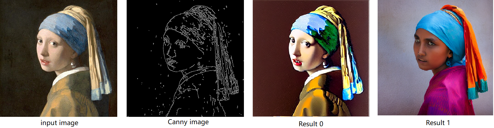
The default iteration is 20, image shape is 512*512, seed is 42, and the input image and prompt is for “Girl with Pearl Earring”. You can adjust or custom your own pipeline attributes for testing.

$ python run_pipe.py

In the case with batch_size=2, the generated image is like below:

‍

Enable LoRA weights for Stable Diffusion

Normal LoRA weights has two types, one is ` pytorch_lora_weights.bin`,the other is using safetensors. In this case, we introduce both methods for these two LoRA weights.

The main idea for LoRA weights enabling, is to append weights onto the original Unet model of Stable Diffusion, then export IR model of Unet which remains LoRA weights.

There are various LoRA models on https://civitai.com/tag/lora , we choose some public models on HuggingFace as an example, you can consider toreplace with your owns.

Step 4-1: Enable LoRA by pytorch_lora_weights.bin

This step introduces the method to add lora weights to Unet model of Stable Diffusion by `pipe.unet.load_attn_procs(...)` function. By using this way, the LoRA weights will be loaded into the attention layers of Unet model of Stable Diffusion.

$ git clone https://huggingface.co/TheUpperCaseGuy/finetune-lora-stable-diffusion
$ rm unet_controlnet.* unet_controlnet/unet_controlnet.onnx
$ python get_model.py -b 2 -sd stable-diffusion-v1-5/ -lt bin -lw finetune-lora-stable-diffusion/

* Remember to delete exist Unet model to generate the new IR with LoRA weights.

Then, run pipeline inference program to check results.

$ python run_pipe.py

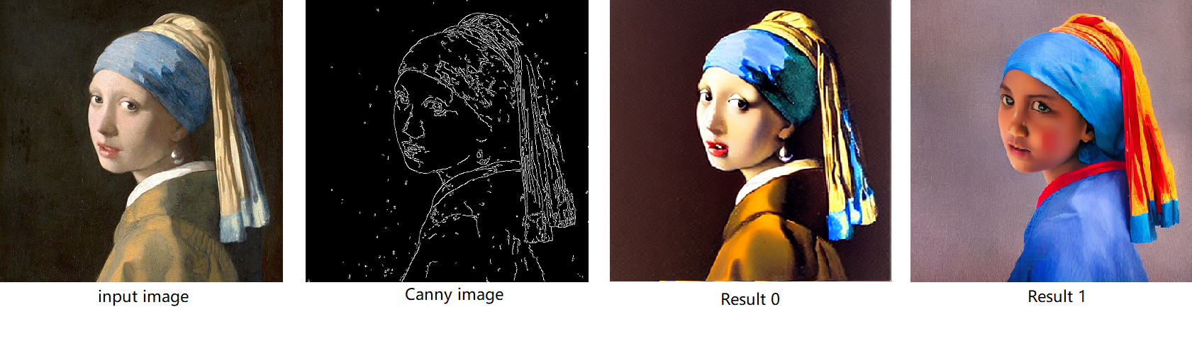
The LoRA weights appended Stable Diffusion model with controlNet pipeline can generate image like below:

Step 4-2: Enable LoRA by safetensors typed weights

This step introduces the method to add LoRA weights to Stable diffusion Unet model by `diffusers/scripts/convert_lora_safetensor_to_diffusers.py`. Diffusers provide the script to generate new Stable Diffusion model by enabling safetensors typed LoRA model. By this method, you will need to replace the weight path to new generated Stable Diffusion model with LoRA. You can adjust value of `alpha` option to change the merging ratio in `W = W0 + alpha * deltaW` for attention layers.

$ git clone https://huggingface.co/ntc-ai/fluffy-stable-diffusion-1.5-lora-trained-without-data
$ git clone https://github.com/huggingface/diffusers.git && cd diffusers
$ python scripts/convert_lora_safetensor_to_diffusers.py --base_model_path ../stable-diffusion-v1-5/ --checkpoint_path ../fluffy-stable-diffusion-1.5-lora-trained-without-data/fluffySingleWordConcept_v10.safetensors --dump_path ../stable-diffusion-v1-5-fluffy-lora --alpha=1.5
$ cd .. && rm unet_controlnet.* unet_controlnet/unet_controlnet.onnx
$ python get_model.py -b 2 -sd stable-diffusion-v1-5-fluffy-lora/ -lt safetensors

Then, run pipeline inference program to check results.

$ python run_pipe.py

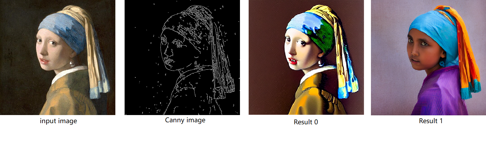
The LoRA weights appended SD model with controlnet pipeline can generate image like below:

Step 4-3: Enable runtime LoRA merging by MatcherPass

This step introduces the method to add lora weights in runtime before Unet or text_encoder model compiling. It will be helpful to client application usage with multiple different LoRA weights to change the image style by reusing the same Unet/text_encoder structure.

This method is to extract lora weights in safetensors file and find the corresponding weights in Unet model and insert lora weights bias. The common method to add lora weights is like:

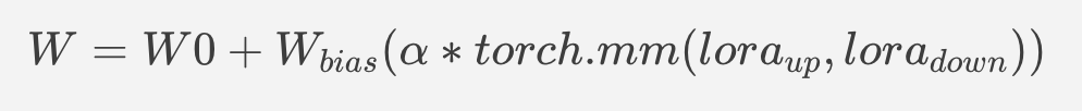
W = W0 + W_bias(alpha * torch.mm(lora_up, lora_down))

I intend to insert Add operation for Unet's attentions' weights by OpenVINO™ `opset10.add(W0,W_bias)`. The original attention weights in Unet model is loaded by `Const` op,  the common processing path is `Const->Convert->Matmul->...`, if we add the lora weights, we should insert the calculated lora weight bias as `Const->Convert->Add->Matmul->...`. In this function, we adopt `openvino.runtime.passes.MatcherPass` to insert `opset10.add()` with call_back() function iteratively.

‍

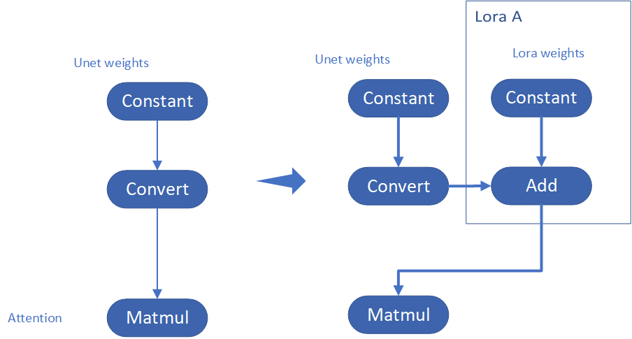
Your own transformation operations will insert opset.Add() firstly, then during the model compiling with device. The graph will do constant folding to combine the Add operation with following MatMul operation to optimize the model runtime inference. Thus, this is an effective method to merge LoRA weights onto original model.

You can check with the implementation source code, and find out the definition of the MatcherPass function called `InsertLoRA(MatcherPass)`:

class InsertLoRA(MatcherPass):
    def __init__(self,lora_dict_list):
        MatcherPass.__init__(self)
        self.model_changed = False

        param = WrapType("opset10.Convert")

        def callback(matcher: Matcher) -> bool:
            root = matcher.get_match_root()
            root_output = matcher.get_match_value()
            for y in lora_dict_list:
                if root.get_friendly_name().replace('.','_').replace('_weight','') == y["name"]:
                    consumers = root_output.get_target_inputs()
                    lora_weights = ops.constant(y["value"],Type.f32,name=y["name"])
                    add_lora = ops.add(root,lora_weights,auto_broadcast='numpy')
                    for consumer in consumers:
                        consumer.replace_source_output(add_lora.output(0))

                    # Use new operation for additional matching
                    self.register_new_node(add_lora)

            # Root node wasn't replaced or changed
            return False

        self.register_matcher(Matcher(param,"InsertLoRA"), callback)

The `InsertLoRA(MatcherPass)` function will be registered by `manager.register_pass(InsertLoRA(lora_dict_list))`, and invoked by `manager.run_passes(ov_unet)`. After this runtime MatcherPass operation, the graph compile with device plugin and ready for inference.

Run pipeline inference program to check the results. The result is same as Step 4-2.

python run_pipe.py -lp fluffy-stable-diffusion-1.5-lora-trained-without-data/fluffySingleWordConcept_v10.safetensors -a 1.5

The LoRA weights appended Stable Diffusion model with controlNet pipeline can generate image like below:

Step 4-4: Enable multiple LoRA weights

There are many different methods to add multiple LoRA weights. I list two methods here. Assume you have two LoRA weigths, LoRA A and LoRA B. You can simply follow the Step 4-3 to loop the MatcherPass function to insert between original Unet Convert layer and Add layer of LoRA A. It's easy to implement. However, it is not good at performance.

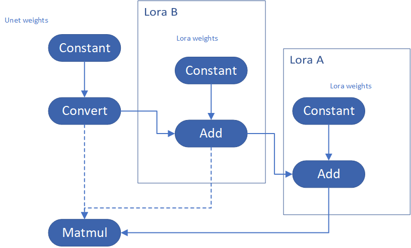
Please consider about the Logic of MatcherPass function. This fucntion required to filter out all layer with the Convert type, then through the condition judgement if each Convert layer connected by weights Constant has been fine-tuned and updated in LoRA weights file. The main costs of LoRA enabling is costed by InsertLoRA() function, thus the main idea is to just invoke InsertLoRA() function once, but append multiple LoRA files' weights.

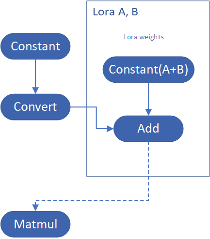
By above method to add multiple LoRA, the cost of appending 2 or more LoRA weights almost same as adding 1 LoRA weigths.

Now, let's change the Stable Diffusion with dreamlike-anime-1.0 to generate image with styles of animation. I pick two LoRA weights for SD 1.5 from https://civitai.com/tag/lora.

• soulcard: https://civitai.com/models/67927?modelVersionId=72591
• epi_noiseoffset: https://civitai.com/models/13941/epinoiseoffset

You probably need to do prompt engineering work to generate a useful prompt like below:

• prompt: "1girl, cute, beautiful face, portrait, cloudy mountain, outdoors, trees, rock, river, (soul card:1.2), highly intricate details, realistic light, trending on cgsociety,neon details, ultra realistic details, global illumination, shadows, octane render, 8k, ultra sharp"
• Negative prompt: "3d, cartoon, lowres, bad anatomy, bad hands, text, error"
• Seed: 0
• num_steps: 30
• canny low_threshold: 100

$ python run_pipe.py -lp soulcard.safetensors -a 0.7 -lp2 epi_noiseoffset2.safetensors -a2 0.7

You can get a wonderful image which generate an animated girl with soulcard typical border like below:

Additional Resources

Download OpenVINO™

OpenVINO™ Documentation

OpenVINO™ Notebooks

Provide Feedback & Report Issues

Notices & Disclaimers

Intel technologies may require enabled hardware, software, or service activation.

No product or component can be absolutely secure.

Your costs and results may vary.

Intel does not control or audit third-party data. You should consult other sources to evaluate accuracy.
Intel disclaims all express and implied warranties, including without limitation, the implied warranties of merchantability, fitness for a particular purpose, and non-infringement, as well as any warranty arising from course of performance, course of dealing, or usage in trade.

No license (express or implied, by estoppel or otherwise) to any intellectual property rights is granted by this document.

© Intel Corporation. Intel, the Intel logo, and other Intel marks are trademarks of Intel Corporation or its subsidiaries. Other names and brands may be claimed as the property of others.

‍

Encrypt Your Dataset and Train Your Model with It Directly

‍Introduction

When we deal with dataset for creating AI models, we need to consider sensitive information managed and stored online in the cloud or on connected devices. Unsecured datasets can be vulnerable to unauthorized access, theft, and misuse, particularly when processed for machine learning workloads. Certain fields, such as industrial or medical sectors, face exceptionally high risks when their data is exposed to these potential threats. For example, if a dataset used to train a detection model for identifying factory process errors is leaked, it can expose sensitive factory process technology. This highlights the importance of safeguarding datasets at every stage, from data storage to model training.

Dataset Management Framework (Datumaro) offers a dataset encryption feature for AI model training. With Datumaro, you can encrypt datasets of any computer vision data format into the DatumaroBinary format. This encrypted dataset can remain encrypted as far as it is needed for decryption. By combining the encrypted dataset with OpenVINO training extensions™, you can use it directly for model training without decryption. Whenever needed, you can use Datumaro once again to decrypt the dataset and convert it back to any major computer vision data format, such as VOC, COCO, or YOLO. Please refer to another posting data_convert for data convert.

Encrypt Your Dataset Using Datumaro

Datumaro provides two ways to encrypt a dataset: CLI and Python API. First, you need to install Datumaro on your system. Please refer to the installation guide here for detailed instructions. Once you have completed the installation of Datumaro, let's first look at the CLI usage. You can encrypt a dataset using the datum convert CLI command as follows:

datum convert -i [input-dataset-path] -o [output-dataset-path] -f datumaro_binary -- --save-media --encryption

The necessary user inputs for this command are as follows:

1. -i <input-dataset-path>: Enter the path to the dataset you want to encrypt in <input-dataset-path>.
2. -o <output-dataset-path>: Enter the path where the encrypted dataset will be produced in <output-dataset-path>.

NOTE:: (Optional) You can additionally specify the data format of your input dataset by entering the -if <input-dataset-format> argument. In most cases, Datumaro can automatically infer the data format of the input dataset, but it might fail. In such cases, you can use the datum detect --show-rejections <input-dataset-path> command to identify the cause of the failure while inferring the data format.

NOTE:: The --save-media argument is a flag that allows you to convert your media files (e.g., images) as well. If this argument is not provided, the encrypted media will not be included in the output directory and only the encrypted annotations are included in the output directory.

Next, let's take a look at how to encrypt a dataset using the Python API. Please examine the following code snippet:

from datumaro import Dataset 

dataset = Dataset.import_from(path="[input-dataset-path]")
dataset.export(save_dir="[output-dataset-path]", 
    format="datumaro_binary", 
    encryption=True, 
    save_media=True,)

You import the dataset by specifying the path of the input dataset in the import_from function as path="<input-dataset-path>". Then, to export the dataset, you specify the path of the output dataset in the save_dir="<output-dataset-path>" of the export function. Similarly, you also need to provide the encryption=True and format="datumaro_binary" keyword arguments as in the CLI example. A more detailed end-to-end example for this can be found in a Jupyter notebook. Please refer to this link for more information.

So far, all the examples have used the datumaro_binary (DatumaroBinary) format for the exported dataset. Currently, the dataset encryption feature is only supported for the datumaro_binary format. DatumaroBinary is a Datumaro's own data format that stores annotation data in binary representation. It is much faster and storage efficient compared to string-based datasets such as COCO based on JSON. For more detailed information about DatumaroBinary, please refer to this link.

How Datumaro Encrypts Your Dataset?

Datumaro uses the Fernet symmetric encryption recipe provided by the cryptography library to encrypt the dataset. Fernet is built on top of a number of standard cryptographic primitives such as AES or HMAC, and hence Fernet guarantees that a message encrypted cannot be manipulated or read without the key. Please refer to this link for detailed information.

When encrypting the dataset, Datumaro generates a secret key through Fernet and saves it as a txt file at the following path: <output-dataset-path>/secret_key.txt. The secret key generated at this path is a 50-characters string, which consists of a randomly generated 32-bytes string encoded in base64, with the prefix datum- added.

cat [output-dataset-path]/secret_key.txt

# A secret key will be randomly generated.
datum-IedFogo3TiyVKF2V1-jT2aO-_r3lWHNQoCWvGEyyjKo=

If you have checked the secret key in this file, you must ensure that it is not in the same location with the dataset. If this secret key is uncovered, an attacker would be able to access the contents of the encrypted dataset. Additionally, this secret key is required when training models using OpenVINO training extensions™ with the encrypted dataset or when decrypting it later. Therefore, you should be careful not to lose this secret key.

The following table briefly shows how the data is encrypted. The binary representation of the data is encrypted, so that the following image cannot be seen by the image viewer.

Train Your Model with the Encrypted Dataset Using OpenVINO Training Extensions™

OpenVINO training extensions™ is a tool that allows convenient training of computer vision models and accelerated inference on Intel® devices by exporting trained models to OpenVINO Intermediate Representation (IR) through a CLI. Within the OpenVINO ecosystem, Datumaro is integrated with OpenVINO training extensions™ as a dataset interface. Therefore, the encrypted dataset can be directly used for model training through OpenVINO training extensions™. For detailed installation instructions of OpenVINO training extensions™, please refer to the following link.

Next, let's explore how to use the encrypted dataset directly for model training through the CLI command.

otx train [template] --train-data-roots [encrypted-dataset-path] --val-data-roots [encrypted-dataset-path] --encryption-key [secret-key]

The user inputs required for this command are as follows:

1. --train-data-roots <encrypted-dataset-path> and --val-data-roots <encrypted-dataset-path>: Specify the path to the encrypted dataset by replacing <encrypted-dataset-path>. Since the DatumaroBinary format uses the same root directory for both the training and validation subsets, both arguments should have the same value.
2. --encryption-key <secret-key>: Provide the secret key corresponding to the encrypted dataset in <secret-key>. This is the 50-character string with the datum- prefix described in the previous section.

NOTE:: <template> is the name of the model template provided by OpenVINO training extensions™. A model template is a recipe for a deep learning model for a specific computer vision task. To explore all the model templates supported by OpenVINO training extensions™, you can use the otx find CLI command or refer to this link.

Decrypt the Encrypted Dataset Using Datumaro

If you want to utilize the encrypted dataset in another AI workload, you need to decrypt the encrypted data. This process reverses the dataset encryption using Datumaro, and encryption-decryption preserves all the information without loss. Similar to the previous section, decryption can be done using the CLI or Python API. Let's first look at decryption using the CLI.

datum convert -i [encrypted-dataset-path] -o [output-dataset-path] -f [output-data-format] --encryption-key [secret-key] --save-media

You can use the same datum convert command as before. However, specify the path to the encrypted dataset as the input dataset path (-i <encrypted-dataset-path>), and provide the secret key, which is a 50-character string with the datum- prefix described in the previous section, as the <secret-key> argument for --encryption-key <secret-key>. Additionally, you can choose any data format supported by Datumaro as the output data format. To learn more about the data formats supported by Datumaro, refer to this link.

Next, let's see how decryption can be done using Python API.

from datumaro import Dataset

dataset = Dataset.import_from(
    path="[encrypted-dataset-path]",
    encryption_key=""
)
dataset.export(
    save_dir="[output-dataset-path]",
    format="[output-data-format]",
    save_media=True
)

Similar to the CLI method, provide the path to the encrypted dataset and the secret key as arguments to the import_from function. For the export function, specify the output dataset path and the output data format.

Conclusion

This post introduced dataset encryption feature provided by Datumaro. It demonstrated how to encrypt a dataset using Datumaro and train a model with the encrypted dataset using OpenVINO training extensions™. Whenever needed you can decrypt it with Datumaro for other AI projects and training frameworks. You can refer to the end-to-end Jupyter notebook example provided on this blog post here for step-by-step guide. The features introduced in this post are available in Datumaro version 1.4.0 or higher and OpenVINO training extensions™ version 1.4.0 or higher.

Datumaro offers a range of useful features for managing datasets besides the dataset encryption feature. You can find examples of other Datumaro features, such as noisy label detection during training with OpenVINO training extensions™, in the Jupyter examples directory. For more information about Datumaro and its capabilities, you can visit the Datumaro documentation page. If you have any questions or requests about using Datumaro, feel free to open an issue here.

Introduction

What is AquilaChat-7B Language Model?

Aquila Language Model is a set of open-source large language models (LLMs) developed by the Beijing Academy of Artificial Intelligence (BAAI). Aquila models support both Chinese and English, commercial license agreements, and compliance with Chinese domestic data regulations.

AquilaChat-7B is a conversational language model that supports Chinese and English dialogue. It is based on the Aquila-7B foundation model and fine-tuned using supervised fine-tuning (SFT). AquilaChat-7B original Pytorch model and configurations are publicly available here.

Hugging Face Optimum Intel

Hugging Face is one of the most popular open-source data science and machine learning platforms. It acts as a hub for AI experts and enthusiasts—like a GitHub for AI. Over 200,000 models are available across Natural language processing, Multimodal models, Computer Vision, and Audio domains.

Hugging Face provides wide support for model optimization and deployment of open-sourced LLMs such as LLaMA, Bloom, GPT-Neox, Dolly 2.0, to name a few. More details please refer to Open LLM Leaderboard.

Optimum-Intel provides a simple interface between the Hugging Face and OpenVINO^TM ecosystem to leverage high-performance inference capabilities for Intel architecture.  Here is a simple example to show how to run Dolly 2.0 models with OVModelForCausalLM using OpenVINO^TM runtime.

from optimum.intel import OVModelForCausalLM
from transformers import AutoTokenizer

model_id = "databricks/dolly-v2-3b"
tokenizer = AutoTokenizer.from_pretrained(model_id)
model = OVModelForCausalLM.from_pretrained(model_id, export=True, use_cache=True)
prompt = "Deep learning is a type of machine learning"
inputs = tokenizer(prompt, return_tensors="pt")
output_ids = model.generate(**inputs)

Hola! So, for LLMs already supported by Hugging Face transformers and optimum, we can smoothly switch the model inference backend from Pytorch to OpenVINO^TM by changing only two lines of code.

However, what if an LLM from an open-source community that not native supported by Hugging Face Transformers library? How can we still leverage the tools of Hugging Face and OpenVINO^TM ecosystem for model optimization and deployment?

Indeed, AquilaChat-7B is a custom model for the Hugging Face Transformers. So, we use it as an example to elaborate the custom model enabling methodology step by step.

How to Enable a Custom Model on Hugging Face?

To leverage the Hugging Face ecosystem and optimization for AquilaChat-7B model, we need to convert the original Pytorch model to Hugging Face Format. Before we dive into conversion details, we need to figure out what is AquilaChat-7B’s model structure, tokenizer, and configurations.

According to Aquila’s official model description:

“The Aquila language model inherits the architectural design advantages of GPT-3 and LLaMA, replacing a batch of more efficient underlying operator implementations and redesigning the tokenizer for Chinese-English bilingual support. The Aquila language model is trained from scratch on high-quality Chinese and English corpora. “

Model Structure and Tokenizer

For model structure, Aquila Model adopts the original Meta LLaMA pytorch implementation, which combines RMSNorm (GPT-3) to improve training stability and Rotary Position Embedding (GPT-NeoX)to incorporate explicit relative position dependency in self-attention.

For tokenizer, instead of using byte-pair encoding (BPE) algorithms implemented by Sentence Piece, Aquila re-trained HuggingFace GPT-NeoX tokenizer with extended vocabulary (vocab_size =100008, including 8 special tokens, e.g. bos_token=100006, eos_token=100007, unk=0, pad=0 used for inference based on here.

Rotary Position Embedding

Rotary Position Embedding (RoPE) encodes the absolute position with a rotation matrix and meanwhile incorporates the explicit relative position dependency in the self-attention formulation. Compare to other position embedding methods, RoPE provides valuable properties such as flexibility of sequence length, long-term decay, and linear self-attention with relative position embedding. Based on the original paper, there are two mainstream implementations of RoPE:

As show in Figure 3, Meta LLaMA’s implementation directly use complex number to calculate rotary position embedding.

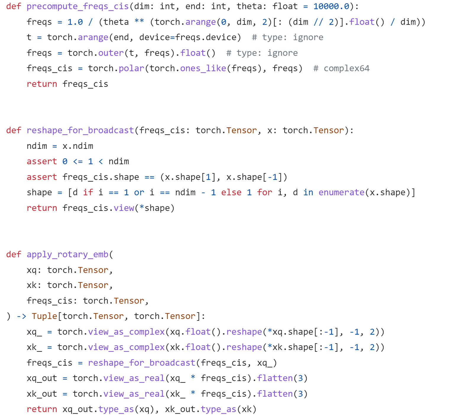
As show in Figure 4, Google PaLM’s implementation expands the complex number operation and calculate sinusoidal functions in matrix equation of real numbers.

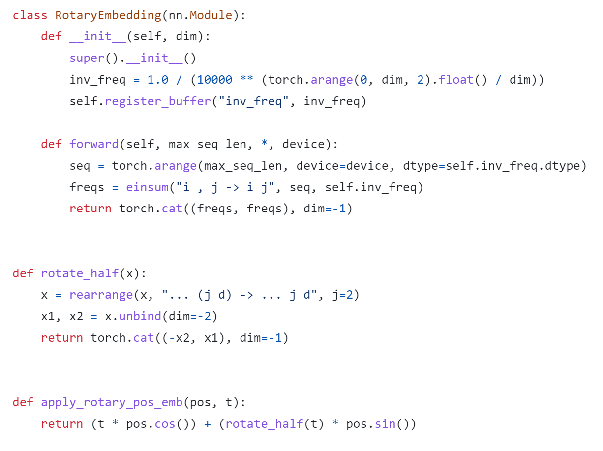
Both RoPE implementations are valid for the Pytorch model. Hugging Face LLaMA implementation adopts PaLM’s RoPE implementation due to the limitation of complex type support for ONNX export.

Besides, Hugging Face provides a useful script convert_llama_weights_to_hf.py to convert the original Meta LLaMA Pytorch Model to Hugging Face Format as follows:

• Extract Pytorch weights and convert Meta LlaMA RoPE implementation to Hugging Face RoPE implementation.
• Convert tokenizer.model trained with Sentence Piece to Hugging Face LLaMA tokenizer.

‍

Convert AquilaChat-7B Model to Hugging Face Format

Similarly, we provide a convert_aquila_weights_to_hf.py to convert AquilaChat-7B Model to Hugging Face Format.

• Extract Pytorch weights and convert Aquila RoPE implementation to Hugging Face RoPE implementation
• Initialize and save a Hugging Face GPT-NeoX Tokenizer with extended vocabulary based on original tokenizer configurations provided by Aquila.
• Add a modeling_aquila.py to enable support forAutoModelForCausalLM and AutoTokenizer

Here is the converted Hugging Face version of AquilaChat-7B v0.6 model uploaded in Hugging Face.

You may convert pytorch weights to Hugging Face format in two steps:

1. Download AquilaChat-7B Pytorch Model and configurations here
2. Convert AquilaChat-7B Pytorch Model and configurations to Hugging Face Format

pip install transformers>=4.30.2
python convert_aquila_weights_to_hf.py --input_dir checkpoints/aquilachat-7b --model_size 7B --output_dir aquilachat-7b-hf

Hugging Face AquilaChat-7B Demo

Setup Environment

pip install optimum==1.8.8 optimum-intel[openvino]==1.9.1 onnx onnxruntime

Run inference with AutoModelForCausalLM

import torch
from transformers import AutoTokenizer, AutoModelForCausalLM
tokenizer = AutoTokenizer.from_pretrained('sammysun0711/aquilachat-7b-hf')
model = AutoModelForCausalLM.from_pretrained('sammysun0711/aquilachat-7b-hf', trust_remote_code=True)
model = model.eval()

question = '北京为什么是中国的首都？'
prompt = (
    '''A chat between a curious human and an artificial intelligence assistant. The assistant gives helpful, detailed, and polite answers to the human's questions.'''
    f'''###Human: {question}###Assistant:'''
)
with torch.no_grad():
    ret = model.generate(
        **tokenizer(prompt, return_tensors='pt').to('cpu'),
        do_sample=False,
        max_new_tokens=200,
        use_cache=True
    )
    print(tokenizer.decode(ret.tolist()[0]))

北京是中国的首都，是因为它在中国历史和文化中具有重要的地位，被选中作为中国的政治中心。在中国古代，北京是几个朝代的首都，如辽、金、元、明、清朝。在这些朝代，北京都是政治、经济、文化中心和军事重镇。此外，北京还是现代中国的政治中心，有着重要的国际地位。

Run inference with OVModelForCausalLM

from transformers import AutoTokenizer
from optimum.intel import OVModelForCausalLM

tokenizer = AutoTokenizer.from_pretrained('sammysun0711/aquilachat-7b-hf')
model = OVModelForCausalLM.from_pretrained('sammysun0711/aquilachat-7b-hf', export=True, use_cache=True, trust_remote_code=True)

question = '北京为什么是中国的首都？'
prompt = (
    '''A chat between a curious human and an artificial intelligence assistant. The assistant gives helpful, detailed, and polite answers to the human's questions.'''
    f'''###Human: {question}###Assistant:'''
)
ret = model.generate(
        **tokenizer(prompt, return_tensors='pt').to('cpu'),
        do_sample=False,
        max_new_tokens=200,
        use_cache=True
)
print(tokenizer.decode(ret.tolist()[0]))

北京是中国的首都，是因为它在中国历史和文化中具有重要的地位，被选中作为中国的政治中心。在中国古代，北京是几个朝代的首都，如辽、金、元、明、清朝。在这些朝代，北京都是政治、经济、文化中心和军事重镇。此外，北京还是现代中国的政治中心，有着重要的国际地位。

Conclusion

In this blog, we show how to convert a custom Large Language Model (LLM) to Hugging Face format to leverage efficient optimization and deployment with Hugging Face and OpenVINO^TM Ecosystem.

Please note, this is the initial model enabling step for AquilaChat-7B model with OpenVINO^TM. We will continue to optimize performance along with upgrading OpenVINO^TM for LLM scaling.  Please refer to OpenVINO^TM and Optimum-Intel official release to get latest efficient support for LLMs with OpenVINO^TM backend.

Reference

• ‍FlagAI AquilaChat-7B
• ‍AquilaChat-7B Hugging Face Model
• ‍Hugging Face Optimum Intel
• ‍LLaMA:Open and Efficient Foundation Language Models
• ‍RoFormer:Enhanced Transformer with Rotary Position Embedding
• ‍RotaryEmbeddings: A Relative Revolution

‍

Authors: Zhen Zhao(Fiona), Cheng Luo, Tingqian Li, Wenyi Zou

Introduction

Since the Large Language Models (LLMs) become the hot topic, a lot Chinese language models have been developed and actively deployed in optimization platforms. chatGLM is one of the popular Chinese LLMs which are widely been evaluated. However, ChatGLM model is not yet a native model in Transformers, which means there remains support gap in official optimum. In this blog, we provide a quick workaround to re-construct the model structure by OpenVINO™ opset contains custom optimized nodes for chatGLM specifically and these nodes has been highly optimized by AMX intrinsic and MHA fusion.

*Please note, this blog only introduces a workaround of optimization method by creating OpenVINO™ stateful model for chatGLM.  This workaround has limitation of platform, which requires to use Intel® 4^th Xeon Sapphire Rapids with AMX optimization. We do not promise the maintenance of this workaround.

Source link: https://github.com/luo-cheng2021/openvino/tree/luocheng/chatglm_custom/tools/gpt

To support more LLMs, including llama, chatglm2, gpt-neox/dolly, gpt-j and falcon. You can refer this link which not limited on SPR platform, also can compute from Core to Xeon:

Source link: https://github.com/luo-cheng2021/ov.cpu.llm.experimental

‍

ChatGLM model brief

If we check with original model source of chatGLM, we can find that the ChatGLM is not compatible with Optimum ModelForCasualML, it defines the new class ChatGLMForConditionalGeneration. This model has 3 main modules (embedding, GLMBlock layers and lm_logits) during the pipeline loop, the structure is like below:

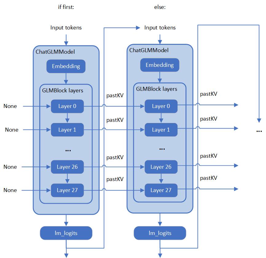
As you can see, the whole pipeline actually require model with two different graphs, the first-time inference with input prompt tokens do not require KV cache as inputs for GLMBlock layers. Since the second iteration, the previous results of QKV Attention should become the inputs of current round model inference. Along with the length of generated token increased, there will remain a lot of large sized memory copies between model inputs and outputs during pipeline inference.  We can use ChatGLM6b default model configurations as an example, the memory copies between input and output arrays are like below pseudocode:

while(eos_token_id || max_seq_len){
    memcpy(model_inp, model_outp, num_layer*2*sizeof(model_outp)* hidden_size)
    model_outp.push_back(gen_token)
}

Therefore, two topics is the most important:

• How we can optimize model inference pipeline to eliminate memory copy between model inputs and outputs
• How we can put optimization efforts on GLMBlock module by reinvent execution graph

Extremely optimization by OpenVINO™ stateful model

Firstly, we need to analyze the structure of GLMBlock layer, and try to encapsulate a class to invoke OpenVINO™ opset with below workflow. Then serialize the graph to IR model(.xml, .bin).

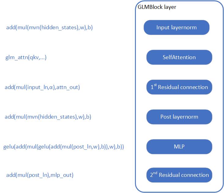
To build an OpenVINO™ stateful model, you can refer to this document to learn.

https://docs.openvino.ai/2022.3/openvino_docs_OV_UG_network_state_intro.html

OpenVINO™ also provide model creation sample to show how to build a model by opset.

https://github.com/openvinotoolkit/openvino/blob/master/samples/cpp/model_creation_sample/main.cpp

It is clear to show that the emphasized optimization block is the custom op of Attention for chatGLM. The main idea is to build up a global context to store and update pastKV results internally, and then use intrinsic optimization for Rotary Embedding and Multi-Head Attentions. In this blog, we provide an optimized the attention structure of chatGLM with AMX intrinsic operators.

At the same time, we use int8 to compress the weights of the Fully Connected layer, you are not required to compress the model by Post Training Quantization (PTQ) or process with framework for Quantization Aware Training(QAT).

Create OpenVINO™ stateful model for chatGLM

Please prepare your hardware and software environment like below and follow the steps to optimize the chatGLM:

Hardware requirements

Intel® 4^th Xeon platform(codename Sapphire Rapids) and above

Software Validation Environment

Ubuntu 22.04.1 LTS

python 3.10.11 for OpenVINO™ Runtime Python API

GCC 11.3.0 to build OpenVINO™ Runtime

cmake 3.26.4

Building OpenVINO™ Source

• Install system dependency and setup environment
• Create and enable python virtual environment

$ conda create -n ov_py310 python=3.10 -y
$ conda activate ov_py310

• Install python dependency

$ pip install protobuf transformers==4.30.2 cpm_kernels torch>=2.0 sentencepiece pandas

• Build OpenVINO™ with GCC 11.3.0
• Clone OpenVINO™ and update submodule

$ git clone https://github.com/luo-cheng2021/openvino.git -b luocheng/chatglm_custom
$ cd openvino && git submodule update --init --recursive

• Install python dependency for building python wheels

$ python -m pip install -U pip 
$ python -m pip install -r ./src/bindings/python/src/compatibility/openvino/requirements-dev.txt
$ python -m pip install -r ./src/bindings/python/wheel/requirements-dev.txt

• Create build directory

$ mkdir build && cd build

• Build OpenVINO™ with CMake

$ cmake .. -DENABLE_LLMDNN=ON \
    -DBUILD_PYTHON_TESTS=ON \
    -DENABLE_CPU_DEBUG_CAPS=OFF \
    -DENABLE_DEBUG_CAPS=OFF  \
    -DCMAKE_BUILD_TYPE=Release \
    -DENABLE_INTEL_MYRIAD_COMMON=OFF \
    -DENABLE_INTEL_GNA=OFF \
    -DENABLE_OPENCV=OFF \
    -DENABLE_CPPLINT=ON \
    -DENABLE_CPPLINT_REPORT=OFF \
    -DENABLE_NCC_STYLE=OFF \
    -DENABLE_TESTS=ON \
    -DENABLE_OV_CORE_UNIT_TESTS=OFF \
    -DENABLE_INTEL_CPU=ON \
    -DENABLE_INTEL_GPU=OFF \
    -DENABLE_AUTO=OFF \
    -DENABLE_AUTO_BATCH=OFF \
    -DENABLE_MULTI=OFF \
    -DENABLE_HETERO=OFF \
    -DENABLE_INTEL_GNA=OFF \
    -DENABLE_PROFILING_ITT=ON\
    -DENABLE_SAMPLES=ON \
    -DENABLE_PYTHON=ON \
    -DENABLE_TEMPLATE=OFF  \
    -DENABLE_OV_ONNX_FRONTEND=OFF \
    -DENABLE_OV_PADDLE_FRONTEND=OFF \
    -DENABLE_OV_PYTORCH_FRONTEND=OFF \
    -DENABLE_OV_TF_FRONTEND=OFF \
    -DENABLE_OPENVINO_DEBUG=OFF \
    -DENABLE_CPU_DEBUG_CAPS=ON \
    -DCMAKE_INSTALL_PREFIX=`pwd`/install \
    -DCMAKE_INSTALL_RPATH=`pwd`/install/runtime/3rdparty/tbb/lib:`pwd`/install/runtime/3rdparty/hddl/lib:`pwd`/install/runtime/lib/intel64 \
    -Dgflags_Dir=`pwd`/../thirdparty/gflags/gflags/cmake
$ make --jobs=$(nproc --all)
$ make install

• Install built python wheel for OpenVINO™ runtime and openvino-dev tools

$ pip install ./install/tools/openvino*.whl

• Check system gcc version and conda runtime gcc version. If the system gcc version is higher than conda gcc version like below, you should update conda gcc version for OpenVINO runtime. (Optional)

##check system (OpenVINO compiling env) gcc version
$ gcc --version
gcc (Ubuntu 11.3.0-1ubuntu1~22.04.1) 11.3.0

##check conda python (runtime env for OpenVINO later) gcc version
$ python
Python 3.10.11 (main, May 16 2023, 00:28:57) [GCC 11.2.0] on linux

##If sys gcc ver > conda gcc ver, upgrade conda gcc ver -> sys gcc ver
$ conda install -c conda-forge gcc=11.3.0

• convert pytorch model to OpenVINO™ IR

$ cd ..
$ python tools/gpt/gen_chatglm.py /path/to/pytorch/model /path/to/ov/IR

Use OpenVINO Runtime API to build Inference pipeline for chatGLM  

We provide a demo by using transformers and OpenVINO™ runtime API to build the inference pipeline. In test_chatglm.py, we create a new class which inherit from transformers.PreTrainedModel. And we update the forward function by build up model inference pipeline with OpenVINO™ runtime Python API. Other member functions are migrated from ChatGLMForConditionalGeneration from modeling_chatglm.py, so that, we can make sure the input preparation work, set_random_seed, tokenizer/detokenizer and left pipelined operation can be totally same as original model source.

To enable the int8 weights compress, you just need a simple environment variable USE_INT8_WEIGHT=1. That is because during the model generation, we use int8 to compress the weights of the Fully Connected layer, and then it can use int8 weights to inference on runtime, you are not required to compress the model by framework or quantization tools.

Please follow below steps to test the chatGLM with OpenVINO™ runtime pipeline:

• Run bf16 model

$ python3  tools/gpt/test_chatglm.py /path/to/pytorch/model /path/to/ov/IR --use=ov

• Run int8 model

$ USE_INT8_WEIGHT=1 python test_chatglm.py /path/to/pytorch/model /path/to/ov/IR --use=ov

‍

Weights compression reduces memory bandwidth utilization to improve inference speed

We use VTune for performance comparison analysis of model weights bf16 and int8. Comparative analysis of memory bandwidth and CPI rate (Table 1). When model weight is compressed to int8, it can reduce memory bandwidth utilization and CPI rate.

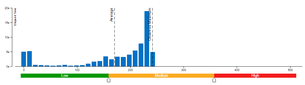
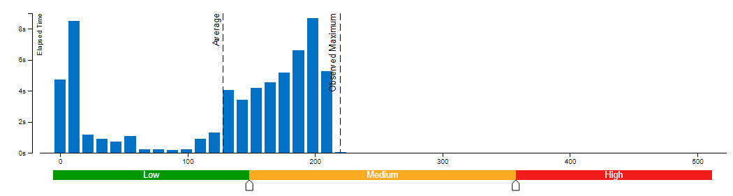
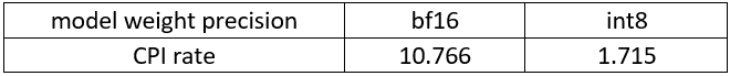
Clockticks per Instructions Retired(CPI) event ratio, also known as Cycles per Instructions, is one of the basic performance metrics for the hardware event-based sampling collection, also known as Performance Monitoring Counter (PMC) analysis in the sampling mode. This ratio is calculated by dividing the number of unhalted processor cycles(Clockticks) by the number of instructions retired. On each processor the exact events used to count clockticks and instructions retired may be different, but VTune Profiler knows the correct ones to use.

A CPI < 1 is typical for instruction bound code, while a CPI > 1 may show up for a stall cycle bound application, also likely memory bound.

Conclusion

Along with the upgrading of OpenVINO™ main branch, the optimization work in this workaround will be generalized and integrated into official release. It will be helpful to scale more LLMs model usage. Please refer OpenVINO™ official release and Optimum-intel OpenVINO™ backend to get official and efficient support for LLMs.

‍

Introduction

In this blog, we will show how to deploy an end-to-end super-resolution pipeline by leveraging OpenVINO^TM Model Server with Demultiplexing in DAG and Custom Node features.

OpenVINO^TM Model Server (OVMS) is a high-performance system for serving models that uses the same architecture and API as TensorFlow Serving and KServe while applying OpenVINO^TM for inference execution. It is implemented in C++ for scalability and optimized for deployment on intel architectures.

Directed Acyclic Graph (DAG) is an OVMS feature that controls the execution of an entire graph of interconnected models defined within the OVMS configuration. The DAG scheduler makes it possible to create a pipeline of models for execution in the server with a single client request.

During the pipeline execution, it is possible to split a request with multiple batches into a set of branches with a single batch. Internally, OVMS demultiplexer will divide the data, process them in parallel and combine the results.

The custom node in OVMS simplifies linking deep learning models into complete pipeline. Custom node can be used to implement all operations on the data which cannot be handled by the neural network model. It is represented by a C++ dynamic library implementing OVMS API defined in custom_node_interface.h.

Super-Resolution Pipeline Workflow

Figure1 shows the super-resolution pipeline in a flowchart, where we use "demultiply_counter=3" without loss of generality. The whole pipeline starts with input data from the Request node via gRPC calls. Batched input data with 5D shape(3,1,3,270,480) is split into a single batch by the DAG demultiplexer. Each single batch of data is fed into a custom node for image preprocessing. The two outputs of the custom node serve as inputs for model A inference. In the end, all inference results are gathered as output C, which will be sent by the Response node to the client via gRPC calls.

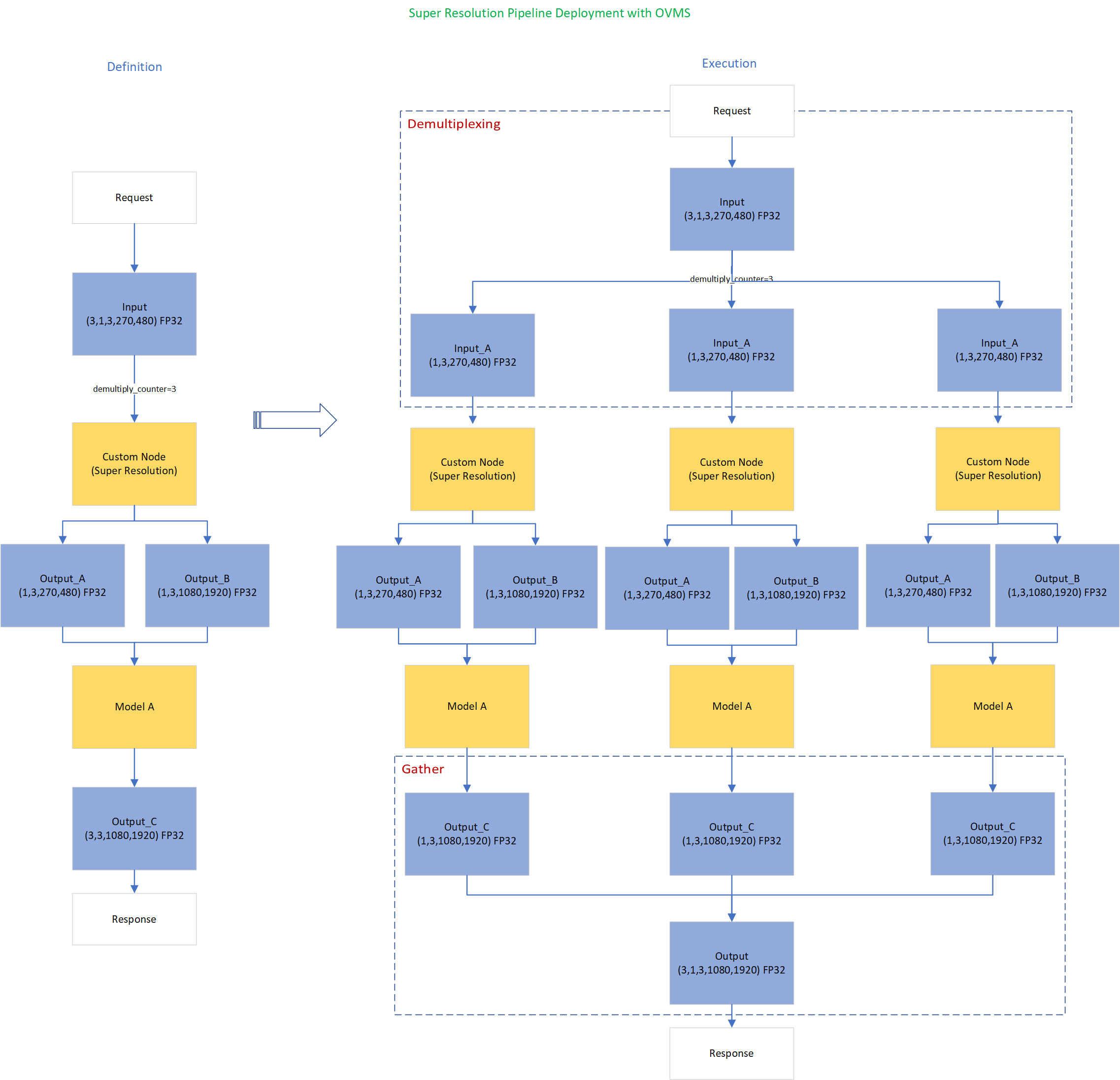
Here is an example configuration for the super-resolution pipeline deployed with OVMS.

{
    "model_config_list": [
        {
            "config": {
                "name": "single-image-super-resolution",
                "base_path": "/models/super_resolution_model_preprocessed/",
                "nireq": 1,
                "plugin_config": {
                    "NUM_STREAMS": "1",
                    "INFERENCE_PRECISION_HINT": "bf16",
                    "AFFINITY": "CORE"
                }
            }
        }
    ],
    "custom_node_library_config_list": [
        {
            "name": "sr_preprocess",
            "base_path": "/models/libcustom_node_super_resolution_nhwc.so"
        }
    ],
    "pipeline_config_list": [
        {
            "name": "super_resolution",
            "inputs": [
                "data"
            ],
            "demultiply_count": -1,
            "nodes": [
                {
                    "name": "sr_preprocess_node",
                    "library_name": "sr_preprocess",
                    "type": "custom",
                    "params": {
                        "image_preprocess_method": "SimpleResize",
                        "debug": "false",
                    },
                    "inputs": [
                        {
                            "image": {
                                "node_name": "request",
                                "data_item": "data"
                            }
                        }
                    ],
                    "outputs": [
                        {
                            "data_item": "out1",
                            "alias": "output1"
                        },
                        {
                            "data_item": "out2",
                            "alias": "output2"
                        }
                    ]
                },
                {
                    "name": "super_resolution_node",
                    "model_name": "single-image-super-resolution",
                    "type": "DL model",
                    "inputs": [
                        {
                            "0": {
                                "node_name": "sr_preprocess_node",
                                "data_item": "output1"
                            }
                        },
                        {
                            "1": {
                                "node_name": "sr_preprocess_node",
                                "data_item": "output2"
                            }
                        }
                    ],
                    "outputs": [
                        {
                            "data_item": "129",
                            "alias": "super_resolution_output"
                        }
                    ]
                }
            ],
            "outputs": [
                {
                    "129": {
                        "node_name": "super_resolution_node",
                        "data_item": "super_resolution_output"
                    }
                }
            ]
        }
    ]
}

“pipeline_config_list” contains super-resolution pipeline information, data enter from the “request” node, flow to “sr_preprocess_node” for image preprocessing, generated two outputs will serve as inputs in “super_resolution_node” for inference, gathered inference results will be returned by “response” node.

• "demultiply_count": acceptable input data batch size when Demultiplexing in DAG feature enabled, “demultiply_count” with value -1 means OVMS can accept dynamic batch input data.

“model_config_list”: contains the basic configuration for super-resolution deep learning model and OpenVINO^TM CPU plugin configuration.

• "nireq": set number of infer requests used in OVMS server for deep learning model
• "NUM_STREAMS": set number of streams used in the CPU plugin
• "INFERENCE_PRECISION_HINT": option to select preferred inference precision in CPU plugin. We can set "INFERENCE_PRECISION_HINT":bf16 on the Xeon platform that supports BF16 precision, such as the 4th Gen Intel® Xeon® Scalable processor (formerly codenamed Sapphire Rapids). Otherwise, we should set "INFERENCE_PRECISION_HINT":f32 as the default value.

‍

“custom_node_library_config_list”: contains the name and path of the custom node dynamic library

Image Preprocessing with libvips in Custom Node

In this blog, we use a single-image-super-resolution model from Open Model Zoo for the super-resolution pipeline. The model requires two inputs according to the model specification. The first input is the original image (shape [1,3,270,480]). The second input is a 4x resized image with bicubic interpolation (shape [1,3,1080,1920]). Both input images expected color space is BGR. Therefore, image preprocessing for input image is required.

Figure2 shows the custom node designed for image preprocessing in the super-resolution pipeline. The custom node takes the original input image as input data. At first, input data is assigned to output 1 without modification. Besides, the input data is resized 4x with bicubic interpolation and assigned as output 2. The two outputs are passed to the model node for inference. For image processing in the custom node, we utilize libvips – an open-source image processing library that is designed to be fast and efficient with low memory usage. Please see the detailed custom node implementation in super_resolution_nhwc.cpp.

Although libvips is very sufficient for image processing operations with less memory, libvips does not provide functionality for layout (NCHW->NHWC) and color space (RGB->BGR) conversion, which is required by the super-resolution model as inputs. Instead, we can integrate layout and color space conversion into models using OpenVINO^TM Preprocessing API.

‍

Integrate Preprocessing with OpenVINO^TM Preprocessing API

OpenVINO^TM Preprocessing API allows adding custom preprocessing steps into the execution graph of OpenVINO^TM models.

Here is a sample code to integrate layout (NCHW-> NHWC) and color space (BRG->RGB) conversion into the super-resolution model with OpenVINO^TM Preprocessing API.

from openvino.runtime import Core, Layout, Type, serialize
from openvino.preprocess import ColorFormat, PrePostProcessor

core = Core()
input_tensor_name_1 = "0"

model_path = "./super_resolution/1/single-image-super-resolution-1032.xml"
model = core.read_model(model_path)
ppp = PrePostProcessor(model)
# Input 1
ppp.input(input_tensor_name_1).tensor().set_element_type(Type.u8)
ppp.input(input_tensor_name_1).tensor().set_color_format(ColorFormat.RGB)
ppp.input(input_tensor_name_1).tensor().set_layout(Layout('NHWC'))
...
model = ppp.build()
serialize(model, 
          './super_resolution_model_preprocessed/1/single-image-super-resolution-1032.xml',
          './super_resolution_model_preprocessed/1/single-image-super-resolution-1032.bin')

In the code snippet above, we first load the original model and initialize the PrePostProcessor object with the original model. Then we modify the model's 1^st input element type to “uint8”, change the color format from the default “BGR” to “RGB”, and set the layout from “NCHW” to “NHWC”. In the end, we build a new model and serialize it on the disk. The whole model preprocessing can be done offline, please find details in model_preprocess.py.

Build Model Server Docker Image for Super-Resolution Pipeline

Build OVMS docker image with custom node

git clone https://github.com/sammysun0711/model_server.git -b super_resolution_demo
cd model_server
IMAGE_TAG_SUFFIX=-sr make docker_build

Copy compiled custom nodes library to the “models” directory

cp src/custom_nodes/lib/ubuntu/libcustom_node_super_resolution_nhwc.so  models/

Setup client environment

cd models
pip install -r requirement.txt
sudo apt-get install libvips libjpeg-turbo8-dev

Integrate preprocessing with OpenVINO^TM Preprocessing API

python model_preprocess.py

The resulting model will be saved in the “super_resolution_model_preprocessed/1” directory.

Super-Resolution Pipeline Demo

Start the OpenVINO^TM Model Server with docker binding with 8 cores

docker run --cpuset-cpus 0-7 --rm -v ${PWD}:/models -p 9001:9001 \
openvino/model_server:latest-sr \
--config_path /models/image_super_resolution_config_nhwc.json \
--port 9001

Run client with command line

python ovms_client_nhwc.py --grpc_port 9001  --input_images_dir images \
--model_name super_resolution --height 270 --width 480 \
--batch_size 1 -niter 100

Figure 3 shows the original input image (shape 270x480).

Figure 4 shows the resized image (shape 1080x1920) after image preprocessing in the custom node.

Figure 5 shows the inference result of the super-resolution model (shape1080x1920).  

Conclusion

In this blog, we demonstrate an end-to-end super-resolution pipeline deployment with OpenVINO^TM Model Server. The whole pipeline takes dynamic batched images (RGB, NHWC) as input, demultiplexing into single batch data, preprocess with a custom node, runs an inference with a super-resolution model, send gathered inference results to the client in the end.

This blog provides following examples that utilize OpenVINO^TM Model Server and OpenVINO^TM features: 

• Enable OVMS DAG demultiplexing feature
• Provide custom node for image preprocessing using libvips
• Provide sample code for integrating preprocessing into the model with OpenVINO^TM Preprocessing API.
• Support super-resolution end-to-end pipeline with image preprocessing and model inference with OVMS DAG scheduler

This AI pipeline implements zero-copy between SYCL and OpenVINO through the Remote Tensor API of the GPU Plugin.

1. Introduction

The development of SYCL simplifies the use of OpenCL, which can fully exploit the computing power of GPU in the pipeline. Meanwhile, SYCL has more flexibility to do customized pre- and post-processing of OpenVINO. To further optimize the pipeline, developers can use GPU Plugin to avoid the memory copy overhead between SYCL and OpenVINO. The GPU plugin provides the ov::RemoteContext and ov::RemoteTensor interfaces for video memory sharing and interoperability with existing native APIs, such as OpenCL, Microsoft DirectX, or VAAPI. For details, please refer to the online documentation of OpenVINO.

Based on the pseudocode of the online documentation, here we provide a simple pipeline sample with Remote Tensor API. Because in the rapid iteration of oneAPI, sometimes customers need quick verification so that this sample can be used for testing. OneAPI also provides a real-world, end-to-end example, which optimizes PointPillars for lidar object detection.

2. Components

SYCL preprocessing is based on the Sepia Filter sample, which demonstrates how to convert a color image to a Sepia tone image, a monochromatic image with a distinctive Brown Gray color. The sample program works by offloading the compute-intensive conversion of each pixel to Sepia tone using SYCL*-compliant code for CPU and GPU.

OpenVINO inferencing is based on the OpenVINO classification sample, the input from SYCL filtered image in the device will be sent into OpenVINO as a remote tensor without a memory copy.

Remote Tensor API: Create RemoteContext from SYCL pre-processing’s native handle. After model compiling, do memory sharing between the application and GPU plugin with from cl::Buffer to remote tensor.

auto cl_queue = get_native<backend::opencl>(sycl_queue);
auto remote_context = ov::intel_gpu::ocl::ClContext(core, cl_queue);
ov::CompiledModel compiled_model = core.compile_model(model, remote_context);
auto cl_buffers = get_native<backend::opencl>(image_buf_out);
auto remote_tensor = remote_context.create_tensor(ov::element::u8, {batch, input_height, input_width, 3}, cl_buffers);
infer_request.set_tensor(input_tensor_name, remote_tensor);

3. Build Sample on Linux

Download the source code from the link. Prepare the model and images.

To run the sample, you need to specify a model and image:

Use pre-trained models from the Open Model Zoo. The models can be downloaded using the Model Downloader. Use images from the media files collection.

 source setupvars.sh
mkdir build
cd build
cmake ..
make 

Run on Intel NUC Core 11 iGPU with OpenVINO 2022.2 and oneAPI 2022.3.

./intel64/hello_nv12_input_classification_oneAPI../model/FP32/alexnet.xml ../image/dog512.bmp GPU 2

Sample Output:

  Loaded image with a width of 512, a height of 512 and 3 channels
[ INFO ] OpenVINO Runtime version ......... 2022.2.0
[ INFO ] Build ........... 2022.2.0-7713-af16ea1d79a-releases/2022/2
[ INFO ] 
[ INFO ] Loading model files: ../model/FP32/alexnet.xml
Running on Intel(R) Iris(R) Xe Graphics [0x9a49]
---Load model - 1126ms
---Create an infer request - 0.515ms
Use remote tensor API and set_tensor
No 1. do inf: 
---sycl buffer  - 0.005ms
---sycl filter total time - 93.342ms
---kernel time: 0.051822 milliseconds
---Set tensor - 0.138ms
---Run infer req - 4.725ms
---get tensor - 0.062ms

Top 3 results:

Image ../image/dog512.bmp

classid probability label
------- ----------- -----
176     0.4579958   "Saluki, gazelle hound"
212     0.2727944   "English setter"
169     0.0513433   "borzoi, Russian wolfhound"

---sum of inference - 98.268ms
No 2. do inf: 
---sycl buffer  - 0.001ms
---sycl filter total time - 0.582ms
---kernel time: 0.05177 milliseconds
---Set tensor - 0.086ms
---Run infer req - 4.162ms
---get tensor - 0.049ms

Top 3 results:

Image ../image/dog512.bmp

classid probability label
------- ----------- -----
176     0.4579958   "Saluki, gazelle hound"
212     0.2727944   "English setter"
169     0.0513433   "borzoi, Russian wolfhound"

---sum of inference - 4.881ms 

Warning: With the updating of OpenVINO and oneAPI, different versions may cause problems with the tools in the common directory or the new SYCL header name. Please use the same version or debug following the corresponding release instructions.

Authors: Devang Aggarwal, Eddy Kim, Preetha Veeramalai

Choosing the right type of hardware for deep learning tasks is a critical step in the AI development workflow. Here at Intel, we provide developers, like yourself, with a variety of hardware options to meet your compute requirements. From Intel® CPUs to Intel® GPUs, there are a wide array of hardware platforms available to meet your needs. When it comes to inferencing on different hardware, the little things matter. For example, the loading of deep learning models, which can be a lengthy process and can lead to a difficult user experience on application startup.

Are there ways to achieve faster model loading time on such devices?

Short answer is, yes, there are ways; one way is to handle the model loading time. Model loading performs several time-consuming device-specific optimizations and network compilations, which can also result in developers seeing a relatively higher first inference latency. These delays can lead to a difficult user experience during application startup. This problem can be solved through a mechanism called Model Caching. Model Caching solves the issue of model loading time by caching the final optimized model directly into a file. Reusing cached networks can significantly reduce the model loading time.

Model Caching

With OpenVINO 2022.3, model caching is currently implemented as a preview feature. To accelerate first inference latency on Intel® GPU, not only should the kernel source code be compiled in a form that can be executed on the GPU, but also various optimization passes must be performed. Kernel caching reuses only the kernels, but model caching reuses even the output of the optimization passes, so the model loading time can be further reduced. Before model caching, kernel caching was used in the same manner: by setting the CACHE_DIR configuration key to a folder where the cache should be stored. Now, to use the preview feature of model caching, set the OV_GPU_CACHE_MODEL environment variable to 1. Since the extension of the cache file created by kernel caching is “cl_cache” and the extension of the cache file created by model caching is “blob”, it is possible to check whether model caching is activated through this.

Note: Currently this is a preview feature with OpenVINO 2022.3. This feature will be fully available in OpenVINO 2023.0.

Developers can now also leverage this preview feature from OpenVINO™ Toolkit in OpenVINO™ Execution Provider for ONNX Runtime, a product that accelerates inferencing of ONNX models using ONNX Runtime API’s while using the OpenVINO™ toolkit as a backend. With the OpenVINO™ Execution Provider, ONNX Runtime delivers better inferencing performance on the same hardware compared to generic acceleration on Intel® CPU, GPU, and VPU. Additionally, by using model caching, OpenVINO™ Execution Provider can speed up the first inference latency of deep learning models on Intel® GPU.

In OpenVINO™ Execution Provider for ONNX Runtime, the model caching feature can been abled by setting the ONNX Runtime config option ‘use_compiled_network’ to True while using the C++/Python API’s. This config option acts like a switch to enable and disable the model caching feature that saves the final optimized model into a .blob file during the very first inference of the model on Intel® hardware.

The blobs are loaded from a directory named ‘ov_compiled_blobs’ relative to the executable path by default. This path however can be overridden using the ONNX Runtime config option ‘blob_dump_path’ which is used to explicitly specify the path where you would like to dump and load the blobs files from when already using theuse_compiled_network (model caching) setting.

Refer to Configuration Options for more information about using these options.

Conclusion

With the Model Caching feature, the deep learning model loading time should significantly decrease. You can now utilize this feature in both the Intel® Distribution of OpenVINO™ Toolkit and OpenVINO™ Execution Provider for ONNX Runtime and experience better first inference latency for your AI models.

‍

Notices & Disclaimers

Intel technologies may require enabled hardware, software or service activation.

No product or component can be absolutely secure.

Your costs and results may vary.

©Intel Corporation.  Intel, the Intel logo, and other Intel marks are trademarks of Intel Corporation or itssubsidiaries.  Other names and brands maybe claimed as the property of others.  

‍

Authors Kunda Xu, Wenyi Zou

Introduction

In this blog is about How to use DL-streamer to build a complete Media-AI pipeline (Including: Video Access, Media Decode, AI Inference, Media Encode and Result Export). And the pipeline will be accelerated by OpenVINO™ and optimize to run on Flex dGPU(Intel® Data Center Flex dGPU)

Requirement

- DL-streamer
Intel® Deep Learning Streamer (Intel® DL Streamer)Pipeline Framework is an easy way to construct media analytics pipelines using Intel® Distribution of OpenVINO™ Toolkit. It leverages the open source media framework GStreamer to provide optimized media operations and Deep Learning Inference Engine from OpenVINO™ Toolkit to provide optimized inference.

- OpenVINO
OpenVINO™ is an open-source toolkit for optimizing and deploying AI inference which can boost deep learning performance in computer vision, automatic speech recognition, natural language processing and other common task.

- Docker (Optional)
Docker is an open-source platform that enables developers to build, deploy, run, update, and manage containers—standardized, executable components that combine application source code with the operating system (OS) libraries and dependencies required to run that code in any environment.
‍

Install DL-Streamer and OpenVINO™ via Docker

Images for Intel® Data Center GPU Flex Series

Images 2023.0.0-ubuntu22-gpu682* are intended for Intel® Data Center GPU Flex Series and include

1.     Intel®DL Streamer 2023.0.0

2.    OpenVINO™ Toolkit 2023.0.0

3.    Drivers for Intel® Data Center GPU Flex Series, drivers version 682.14

Two images are listed below, images -devel additionally contain samples and development files

Runtime image that includes GStreamer* Pipeline Framework elements, elements built with Intel® oneAPI DPC++/C++ Compiler

docker pull intel/dlstreamer:2023.0.0-ubuntu22-gpu682-dpcpp

Developer image that builds on runtime image containing samples, development files and a model downloader, built with Intel® oneAPI DPC++/C++ Compiler

docker pull intel/dlstreamer:2023.0.0-ubuntu22-gpu682-dpcpp-devel

‍

Taking “dlstreamer:2023.0.0-ubuntu22-gpu682-dpcpp” docker images as a sample to show how to pull the docker image from docker hub.

docker pull intel/dlstreamer:2023.0.0-ubuntu22-gpu682-dpcpp

‍

DL-Streamer Media-AI pipeline quick start example

Make sure the pre-requirement had already installed, there is a very basic introduction to using object detection models(yolov5) to build a DL-streamer pipeline.

Step 1.Download video and yolov5s model file

Download video

curl -L -o people_walking_sample.mp4 https://player.vimeo.com/external/456357349.hd.mp4?s=08ad0b382841957ae4057d880bca5ac1bfdf1172

‍

Download yolov5s-416_INT8 model from pipeline-zoo-models

mkdir yolov5s-416_INT8 && cd yolov5s-416_INT8

wget https://raw.githubusercontent.com/dlstreamer/pipeline-zoo-models/main/storage/yolov5s-416_INT8/FP16-INT8/yolov5s.xml

wget https://github.com/dlstreamer/pipeline-zoo-models/raw/main/storage/yolov5s-416_INT8/FP16-INT8/yolov5s.bin

wget https://raw.githubusercontent.com/dlstreamer/pipeline-zoo-models/main/storage/yolov5s-416_INT8/yolo-v5.json

‍
Step 2.Enter Docker and copy the files into docker container

Create and enter the docker container

docker run -it --device /dev/dri/ --user root --rm intel/dlstreamer:2023.0.0-ubuntu22-gpu682-dpcpp

Open another terminal for file copy into container ,copy video and model into docker container

sudo docker cp yolov5s-416_INT8/ <Docker CONTAINER ID>:/home/dlstreamer

docker cp people_walking_sample.mp4 <Docker CONTAINER ID>:/home/dlstreamer

‍

Step 3. Run an object detection Media-AI pipeline

By the following script, we can run pipeline the Media-AI objection detection on the Flex dGPU in the docker container.

gst-launch-1.0 filesrc location=/path/to/people_walking_sample.mp4 ! decodebin !  capsfilter caps="video/x-raw(memory:VASurface)" ! gvadetect model=/path/to/yolov5s-416_INT8/yolov5s.xml model_proc=/path/to/yolov5s-416_INT8/yolo-v5.json inference-interval=1 device=GPU.0 batch-size=32 pre-process-backend=vaapi-surface-sharing ! queue ! gvatrack tracking-type=short-term-imageless ! gvafpscounter ! fakesink sync=false

If want to encode the detection result and save as video file, can use the follow script

gst-launch-1.0 filesrc location=/path/to/people_walking_sample.mp4 ! decodebin !  capsfilter caps="video/x-raw(memory:VASurface)" ! gvadetect model=/path/to/yolov5s-416_INT8/yolov5s.xml model_proc=/path/to/yolov5s-416_INT8/yolo-v5.json inference-interval=1 device=GPU.0 batch-size=32 pre-process-backend=vaapi-surface-sharing ! queue ! gvatrack tracking-type=short-term-imageless ! meta_overlay device=GPU ! gvafpscounter ! vaapipostproc ! vaapih265enc rate-control=cbr bitrate=6144  ! filesink location=./encoded_video_track.265 sync=false

‍

The encoded video file will save in the container and can be copied out in new terminal.

docker cp <Docker CONTAINER ID>:/home/dlstreamer encoded_video_track.265 .

‍

PS. Instruction about DL-streamer CLI parameter

decodebin: Auto-magically constructs a decoding pipeline using available decoders and demuxers via auto-plugging.

vaapipostproc: Consists in various post processing algorithms to be applied to VA surfaces. For e.g. scaling, deinterlacing (bob, motion-adaptive, motion-compensated), noise reduction or sharpening.

gvadetect: Performs object detection on a full-frame or region of interest (ROI) using object detection models such as YOLO v3-v5, MobileNet-SSD, Faster-RCNN etc. Outputs the ROI for detected objects.

gvatrack: Performs object tracking using zero-term, zero-term-imageless, or short-term-imageless tracking algorithms. Zero-term tracking assigns unique object IDs and requires object detection to run on every frame. Short-term tracking allows to track objects between frames, there by reducing the need to run object detection on each frame. Imageless tracking forms object associations based on the movement and shape of objects, and it does not use image data.

gvafpscounter: Measures frames per second across multiple streams in a single process.

Tuning Tips

Users can refer the different platform using case which were supported by OpenVINO™ and the device profiling API to realize performance tuning of your inference program between CPU, iGPU, dGPU. It will also be helpful to developer finding out the place where has the potential space of performance improvement.

LoRA, or Low-Rank Adaptation, reduces the number of trainable parameters by learning pairs of rank-decompostion matrices while freezing the original weights. This vastly reduces the storage requirement for large language models adapted to specific tasks and enables efficient task-switching during deployment all without introducing inference latency. Thus for a basic large model, the task scenarios of the model can be changed by different LoRAs. In a previous blog, it has been described how to convert the LoRAs-fused base model from pytorch to OpenVINO IR, but this method has the shortcoming of not being able to dynamically switch between LoRAs, which happen to be famous for their flexibility.

This blog will introduce how to implement the dynamic switching of LoRAs in a trick way. Specifically, for most of the tasks, the structure of the base model and LoRAs is unchanged, what changes is the task-specific LoRAs weights, and we can use these LoRAs weights as inputs to the model to achieve the dynamic switching function. All the code involved in this blog can be found here.

‍

‍

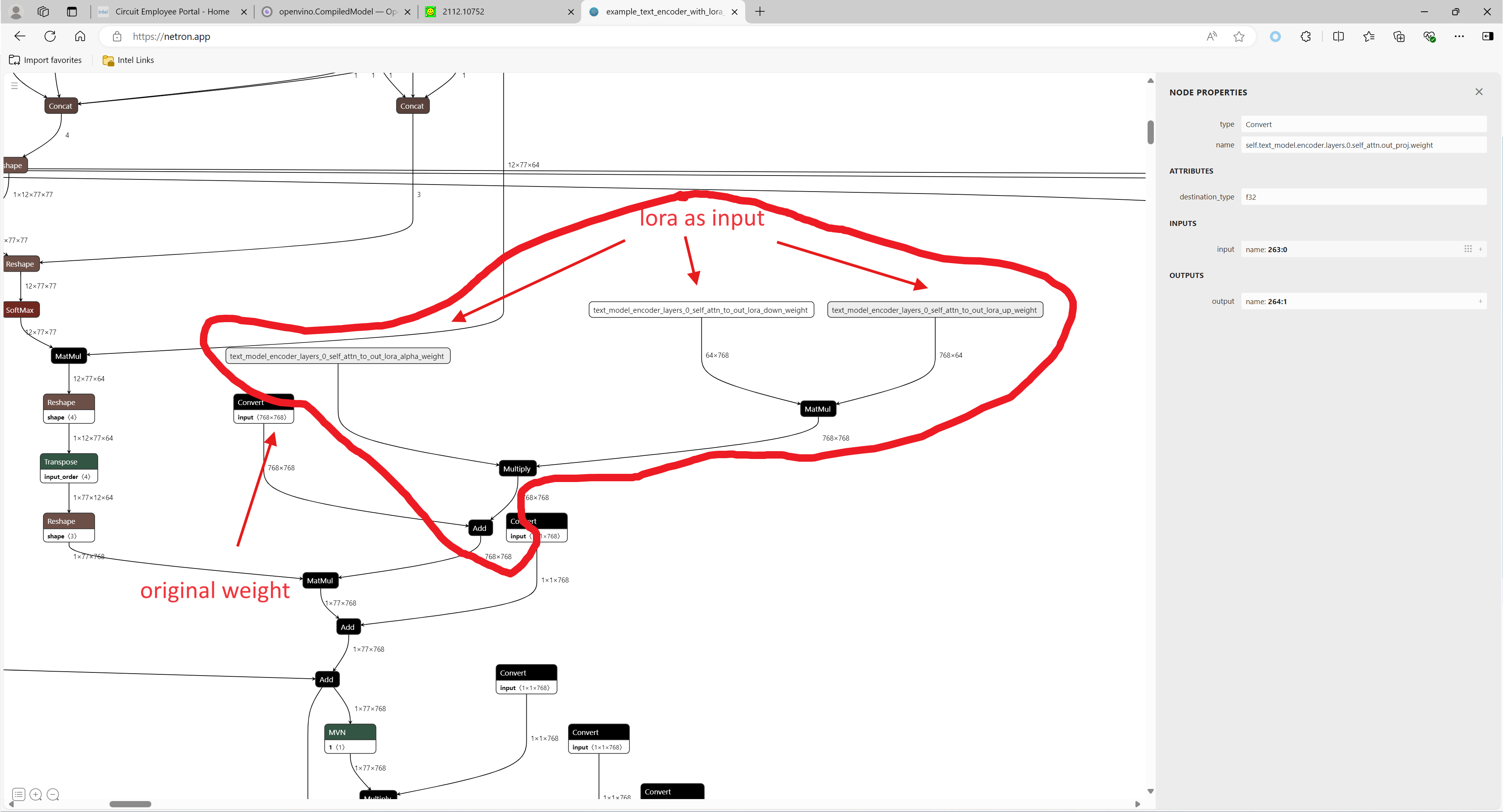
1. Environment preparation

# %python -m venv stable-diffusion-lora
# %source stable-diffusion-lora/bin/activate
git clone https://github.com/TianmengChen/sd1.5_controlnet_lora.git
pip install -r requirements.txt

‍

2. Convert and inference

you should first change the lora file path and configs at first around line 478 in ov_model_export.py, after run python ov_model_ export.py, you will get related OpenVINO IR model. Then you can run ov_model_infer.py.

python ov_model_export.py
python ov_model_infer.py

‍

3. Codes explanation

The most important part is the code in util.py, which is used to modify the model graph and load lora.

Function load_lora(lora_path, DEVICE_NAME) is used to load lora, get lora's shape and weights per layers and modify each layer's name.

‍

def load_lora(lora_path, DEVICE_NAME):
    state_dict = load_file(lora_path)
    if DEVICE_NAME =="CPU":
        for key, value in state_dict.items():
            if isinstance(value, torch.Tensor):
                    value_fp32 = value.type(torch.float32)
                    state_dict[key] = value_fp32

    layers_per_block = 2#TODO
    state_dict = _maybe_map_sgm_blocks_to_diffusers(state_dict, layers_per_block)
    state_dict, network_alphas = _convert_non_diffusers_lora_to_diffusers(state_dict)

    # now keys in format like: "unet.up_blocks.0.attentions.2.transformer_blocks.8.ff.net.2.lora.down.weight"'
    new_state_dict = {}
    for key , value in state_dict.items():
        if len(value.shape)==4:
            # new_value = torch.reshape(value, (value.shape[0],value.shape[1]))
            new_value = torch.squeeze(value)
        else:
            new_value = value
        new_state_dict[key.replace('.', '_').replace('_processor','')] = new_value
    # now keys in format like: "unet_up_blocks_0_attentions_2_transformer_blocks_8_ff_net_2_lora_down_weight"'

    LORA_PREFIX_UNET = "unet"
    LORA_PREFIX_TEXT_ENCODER = "text_encoder"
    LORA_PREFIX_TEXT_2_ENCODER = "text_encoder_2"

    lora_text_encoder_input_value_dict = {}
    lora_text_encoder_2_input_value_dict = {}
    lora_unet_input_value_dict = {}

    lora_alpha = collections.Counter(network_alphas.values()).most_common()[0][0]

    for key in new_state_dict.keys():
        if LORA_PREFIX_TEXT_ENCODER in key and "lora_down" in key and LORA_PREFIX_TEXT_2_ENCODER not in key:
            layer_infos = key.split(LORA_PREFIX_TEXT_ENCODER + "_")[-1]
            lora_text_encoder_input_value_dict[layer_infos] = new_state_dict[key]
            lora_text_encoder_input_value_dict[layer_infos.replace("lora_down", "lora_up")] = new_state_dict[key.replace("lora_down", "lora_up")]

        elif LORA_PREFIX_TEXT_2_ENCODER in key and "lora_down" in key:
            layer_infos = key.split(LORA_PREFIX_TEXT_2_ENCODER + "_")[-1]
            lora_text_encoder_2_input_value_dict[layer_infos] = new_state_dict[key]
            lora_text_encoder_2_input_value_dict[layer_infos.replace("lora_down", "lora_up")] = new_state_dict[key.replace("lora_down", "lora_up")]

        elif LORA_PREFIX_UNET in key and "lora_down" in key:
            layer_infos = key.split(LORA_PREFIX_UNET + "_")[-1]
            lora_unet_input_value_dict[layer_infos] = new_state_dict[key]
            lora_unet_input_value_dict[layer_infos.replace("lora_down", "lora_up")] = new_state_dict[key.replace("lora_down", "lora_up")]

    #now the keys in format without prefix

    return lora_text_encoder_input_value_dict, lora_text_encoder_2_input_value_dict, lora_unet_input_value_dict, lora_alpha

‍

Function add_param(model, lora_input_value_dict) is used to add input parameter per names of related layers, which will be connected to model with manager.register_pass(InsertLoRAUnet(input_param_dict)) and manager.register_pass(InsertLoRATE(input_param_dict)), in these two classes, we search the whole model graph to find the related layers by their names and connect them with lora.

def add_param(model, lora_input_value_dict):
        param_list = []
        for key, value in lora_input_value_dict.items():
            if '_lora_down' in key:
                key_down = key
                key_up = key_down.replace('_lora_down','_lora_up')
                name_alpha = key_down.replace('_lora_down','_lora_alpha')
                lora_alpha = ops.parameter(shape='',name=name_alpha)
                lora_alpha.output(0).set_names({name_alpha})
                # lora_down = ops.parameter(shape=[-1, lora_input_value_dict[key_down].shape[-1]], name=key_down)
                lora_down = ops.parameter(shape=lora_input_value_dict[key_down].shape, name=key_down)
                lora_down.output(0).set_names({key_down})
                # lora_up = ops.parameter(shape=[lora_input_value_dict[key_up].shape[0], -1], name=key_up)
                lora_up = ops.parameter(shape=lora_input_value_dict[key_up].shape, name=key_up)
                lora_up.output(0).set_names({key_up})
                param_list.append(lora_alpha)
                param_list.append(lora_down)
                param_list.append(lora_up)
        model.add_parameters(param_list)

‍

class InsertLoRAUnet(MatcherPass):
    def __init__(self, input_param_dict):
        MatcherPass.__init__(self)
        self.model_changed = False
        param = WrapType("opset10.Convert")

        def callback(matcher: Matcher) -> bool:
            root = matcher.get_match_root()
            root_output = matcher.get_match_value()
            for key in input_param_dict.keys():
                if root.get_friendly_name().replace('.','_').replace('self_unet_','') == key.replace('_lora_down','').replace('to_out','to_out_0'):

                    key_down = key
                    key_up = key_down.replace('_lora_down','_lora_up')
                    key_alpha = key_down.replace('_lora_down','_lora_alpha')

                    consumers = root_output.get_target_inputs()

                    lora_up_node = input_param_dict.pop(key_up)
                    lora_down_node = input_param_dict.pop(key_down)
                    lora_alpha_node = input_param_dict.pop(key_alpha)   

                    lora_weights = ops.matmul(data_a=lora_up_node, data_b=lora_down_node, transpose_a=False, transpose_b=False, name=key.replace('_down',''))
                    lora_weights_alpha = ops.multiply(lora_alpha_node, lora_weights)
                    if len(root.shape)!=len(lora_weights_alpha.shape):
                        # lora_weights_alpha_reshape = ops.reshape(lora_weights_alpha, root.shape, special_zero=False)
                        lora_weights_alpha_reshape = ops.unsqueeze(lora_weights_alpha, axes=[2, 3])
                        add_lora = ops.add(root,lora_weights_alpha_reshape,auto_broadcast='numpy')
                    else:
                        add_lora = ops.add(root,lora_weights_alpha,auto_broadcast='numpy')
                    for consumer in consumers:
                        consumer.replace_source_output(add_lora.output(0))

                    return True
            # Root node wasn't replaced or changed
            return False
        
        self.register_matcher(Matcher(param,"InsertLoRAUnet"), callback)

‍

class InsertLoRATE(MatcherPass):
    def __init__(self, input_param_dict):
        MatcherPass.__init__(self)
        self.model_changed = False
        param = WrapType("opset10.Convert")

        def callback(matcher: Matcher) -> bool:
            root = matcher.get_match_root()
            root_output = matcher.get_match_value()
            root_name = None
            if 'Constant_' in root.get_friendly_name() and root.shape == ov.Shape([768,768]):
                target_input = root.output(0).get_target_inputs()
                for v in target_input:
                    for input_of_MatMul in v.get_node().inputs():
                        if input_of_MatMul.get_shape()== ov.Shape([1,77,768]):
                            Add_Node = input_of_MatMul.get_source_output().get_node()
                            for Add_Node_output in Add_Node.output(0).get_target_inputs():
                                if 'k_proj' in Add_Node_output.get_node().get_friendly_name():
                                    for i in Add_Node_output.get_node().inputs():
                                        if i.get_shape() == ov.Shape([768,768]) and 'k_proj' in i.get_source_output().get_node().get_friendly_name():
                                            root_name = i.get_source_output().get_node().get_friendly_name().replace('k_proj', 'q_proj')

            root_friendly_name = root_name if root_name else root.get_friendly_name()
            
            for key in input_param_dict.keys():
                if root_friendly_name.replace('.','_').replace('self_','') == key.replace('_lora_down','_proj').replace('_to','').replace('_self',''):
                    # print(root_friendly_name)
                    key_down = key
                    key_up = key_down.replace('_lora_down','_lora_up')
                    key_alpha = key_down.replace('_lora_down','_lora_alpha')

                    consumers = root_output.get_target_inputs()

                    lora_up_node = input_param_dict.pop(key_up)
                    lora_down_node = input_param_dict.pop(key_down)
                    lora_alpha_node = input_param_dict.pop(key_alpha)   

                    lora_weights = ops.matmul(data_a=lora_up_node, data_b=lora_down_node, transpose_a=False, transpose_b=False, name=key.replace('_down',''))
                    lora_weights_alpha = ops.multiply(lora_alpha_node, lora_weights)
                    add_lora = ops.add(root,lora_weights_alpha,auto_broadcast='numpy')
                    for consumer in consumers:
                        consumer.replace_source_output(add_lora.output(0))

                    return True
                
            if len(input_param_dict) == 0:
                print("All loras are added")
            # Root node wasn't replaced or changed
            return False
        
        self.register_matcher(Matcher(param,"InsertLoRATE"), callback)

‍

4. GenAI

In addition to this, the latest OpenVINO GenAI provides the Cpp API for LoRA. You can find it here.

‍

‍

Authors: Tianmeng Chen, Xiake Sun

Introduction

Stable Diffusion is a generative artificial intelligence model that produces unique images from text and image prompts. ControlNet is a neural network that controls image generation in Stable Diffusion by adding extra conditions. The specific structure of Stable Diffusion + ControlNet is shown below:

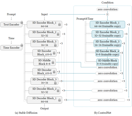
In many cases, ControlNet is used in conjunction with other models or frameworks, such as OpenPose, Canny, Line Art, Depth, etc. An example of Stable Diffusion + ControlNet + OpenPose:

OpenPose identifies the key points of the human body from the left image to get the pose image, and then inputs the Pose image to ControlNet and Stable Diffusion to get the right image. In this way, ControlNet can control the generation of Stable Diffusion.

In this blog, we focus on enabling the stable diffusion pipeline with ControlNet in Optimum-intel. Some details can be found in this open PR.

How to enable StableDiffusionControlNet pipeline in Optimum-Intel

The important code is in optimum/intel/openvino/modelling_diffusion.py and optimum/exporters/openvino/model_configs.py. There is the diffusion pipeline related code in file modelling_diffusion.py, you can find several Class: OVStableDiffusionPipelineBase, OVStableDiffusionPipeline, OVStableDiffusionXLPipelineBase, OVStableDiffusionXLPipeline, and so on. What we need to do is mimic these base classes to add the OVStableDiffusionControlNetPipelineBase, StableDiffusionContrlNetPipelineMixin, and OVStableDiffusionControlNetPipeline. A few of the important parts are as follows:

_from_pretrained function in class OVStableDiffusionControlNetPipelineBase: initial whole pipeline from local or download.

_from_transformers function in class OVStableDiffusionControlNetPipelineBase: convert torch model to OpenVINO IR model.

_reshape_unet_controlnet and _reshape_controlnet in class OVStableDiffusionControlNetPipelineBase: reshape dynamic OpenVINO IR model to static in order to decrease cost.

__call__ function in class StableDiffusionContrlNetPipelineMixin: do the inference in the pipeline.

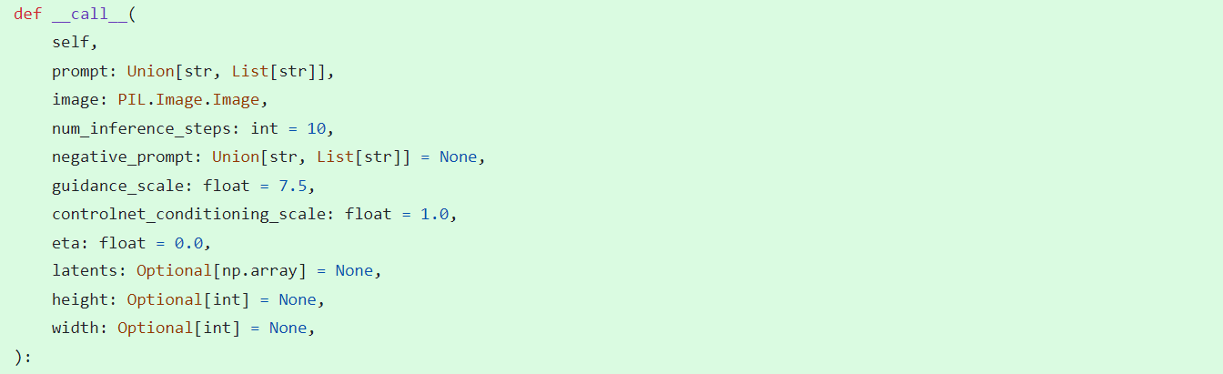
In model_configs.py, we define UNetControlNetOpenVINOConfig by inheriting UNetOnnxConfig, which includes UNetControlNet inputs and outputs.

By now we have completed the rough code, after which some very detailed code additions are needed, so I won't go into that here.

How to use StableDiffusionControlNet pipeline via Optimum-Intel

The next step is how to use the code, examples of which can be found in this repository.

Installation and update of environments and dependencies from source. Make sure your python version is greater that 3.10 and your optimum-intel and optimum version is up to date accounding to the requirements.txt.

# %python -m venv stable-diffusion-controlnet
# %source stable-diffusion-controlnet/bin/activate
%pip install -r requirements.txt

‍

At first, we should convert pytorch model to openvino IR with dynamic shape. Now import related packages.

from optimum.intel import OVStableDiffusionControlNetPipeline
import os
from diffusers import UniPCMultistepScheduler

‍

Set pytroch models of stable diffusion 1.5 and controlnet path if you have them in local, else you can run pipeline from download.

SD15_PYTORCH_MODEL_DIR="stable-diffusion-v1-5"
CONTROLNET_PYTORCH_MODEL_DIR="control_v11p_sd15_openpose"


if os.path.exists(SD15_PYTORCH_MODEL_DIR) and os.path.exists(CONTROLNET_PYTORCH_MODEL_DIR):
    scheduler = UniPCMultistepScheduler.from_config("scheduler_config.json")
    ov_pipe = OVStableDiffusionControlNetPipeline.from_pretrained(SD15_PYTORCH_MODEL_DIR, controlnet_model_id=CONTROLNET_PYTORCH_MODEL_DIR, compile=False, export=True, scheduler=scheduler,device="GPU.1")
    ov_pipe.save_pretrained(save_directory="./ov_models_dynamic")
    print("Dynamic model is saved in ./ov_models_dynamic")  

else:
    scheduler = UniPCMultistepScheduler.from_config("scheduler_config.json")
    ov_pipe = OVStableDiffusionControlNetPipeline.from_pretrained("runwayml/stable-diffusion-v1-5", controlnet_model_id="lllyasviel/control_v11p_sd15_openpose", compile=False, export=True, scheduler=scheduler, device="GPU.1")
    ov_pipe.save_pretrained(save_directory="./ov_models_dynamic")
    print("Dynamic model is saved in ./ov_models_dynamic")

‍

Now you will have openvino IR models file under **ov_models_dynamic ** folder.

from optimum.intel import OVStableDiffusionControlNetPipeline
from controlnet_aux import OpenposeDetector
from pathlib import Path
import numpy as np
import os
from PIL import Image
from diffusers import UniPCMultistepScheduler
import requests
import torch

‍

We recommand to use static shape model to decrease GPU memory cost. Set your STATIC_SHAPE and DEVICE_NAME.

NEED_STATIC = True
STATIC_SHAPE = [1024,1024]
DEVICE_NAME = "GPU.1"

‍

Load openvino model files, if is static, reshape dynamic models to fixed shape.

if NEED_STATIC:
    print("Using static models")
    scheduler = UniPCMultistepScheduler.from_config("scheduler_config.json")
    ov_config ={"CACHE_DIR": "", 'INFERENCE_PRECISION_HINT': 'f16'}
    if not os.path.exists("ov_models_static"):
        if os.path.exists("ov_models_dynamic"):
            print("load dynamic models from local ov files and reshape to static")
            ov_pipe = OVStableDiffusionControlNetPipeline.from_pretrained(Path("ov_models_dynamic"), scheduler=scheduler, device=DEVICE_NAME, compile=True, ov_config=ov_config, height=STATIC_SHAPE[0], width=STATIC_SHAPE[1])
            ov_pipe.reshape(batch_size=1 ,height=STATIC_SHAPE[0], width=STATIC_SHAPE[1], num_images_per_prompt=1)
            ov_pipe.save_pretrained(save_directory="./ov_models_static")
            print("Static model is saved in ./ov_models_static")  
        else:
            raise ValueError("No ov_models_dynamic exists, please trt ov_model_export.py first")
    else:
        print("load static models from local ov files")
        ov_pipe = OVStableDiffusionControlNetPipeline.from_pretrained(Path("ov_models_static"), scheduler=scheduler, device=DEVICE_NAME, compile=True, ov_config=ov_config, height=STATIC_SHAPE[0], width=STATIC_SHAPE[1])
else:
    scheduler = UniPCMultistepScheduler.from_config("scheduler_config.json")
    ov_config ={"CACHE_DIR": "", 'INFERENCE_PRECISION_HINT': 'f16'}
    print("load dynamic models from local ov files")
    ov_pipe = OVStableDiffusionControlNetPipeline.from_pretrained(Path("ov_models_dynamic"), scheduler=scheduler, device=DEVICE_NAME, compile=True, ov_config=ov_config)
     

‍

Set seed for Numpy and torch to make result reproducible.

seed = 42
torch.manual_seed(seed)           
torch.cuda.manual_seed(seed)       
torch.cuda.manual_seed_all(seed)
np.random.seed(seed)

‍

Load image for ControlNet, or you can use your own image, or generate image with OpenPose OpenVINO model, notice that OpenPose model is not supported by OVStableDiffusionControlNetPipeline yet, so you need to convert it to openvino model first manually. Here we use directly the result from OpenPose:

pose = Image.open(Path("pose_1024.png"))

‍

Set prompt, negative_prompt, image inputs.

prompt = "Dancing Darth Vader, best quality, extremely detailed"
negative_prompt = "monochrome, lowres, bad anatomy, worst quality, low quality"

result = ov_pipe(prompt=prompt, image=pose, num_inference_steps=20, negative_prompt=negative_prompt, height=STATIC_SHAPE[0], width=STATIC_SHAPE[1])

result[0].save("result_1024.png")

‍

Introduction

MiniCPM is an End-Side LLM developed by ModelBest Inc. and TsinghuaNLP. MiniCPM-V is a series of end-side multimodal LLMs (MLLMs) designed for vision-language understanding. The models take image and text as inputs and provide high-quality text outputs. MiniCPM-V 2.0 is an efficient version with promising performance for deployment. The model is built based on SigLip-400Mand MiniCPM-2.4B, connected by a perceiver resampler. On this blog, we provide the OpenVINO™ optimization for MiniCPM-V 2.0 on Intel® platforms.

You can find more information on GitHub repository:https://github.com/OpenBMB/MiniCPM-V

OpenVINO™backend on Minicpm-V-2

Step 1: Install system dependency and setup environment

Create and enable python virtual environment

conda create -n ov_py310 python=3.10 -y
conda activate ov_py310

Clone the MiniCPM-V repository from GitHub

git clone https://github.com/wenyi5608/MiniCPM-V.git -b ov_runtime

Chage the current directory to the MiniCPM-V OpenVINO™ Runtime folder

 cd MiniCPM-V/eval_mm/openvinoruntime/

Install python dependency

pip install -r requirement.txt 
pip install --pre -U openvino openvino-tokenizers --extra-index-url https://storage.openvinotoolkit.org/simple/wheels/nightly

Step2: Export to OpenVINO™ models

python ov_convert_minicpm-v-2.py -m /path/to/ openbmb/MiniCPM-V-2 -o /path/to/ MiniCPM-V-2 _ov

Step3: Simple inference test with OpenVINO™

python ov_minicpm-v2-test.py -m /path/to/ MiniCPM-V-2 _ov -pic /path/to/hk_OCR.jpg -p “Describe the content of the image” 

Question: Describe the content of the image

Answer:

The image captures the vibrant and bustling atmosphere of abusy city street in Hong Kong. The street is lined with an array of neon signsand billboards, each one advertising a different business or establishment. Thesigns are in a variety of languages, including English, Chinese, and Japanese,reflecting the multicultural nature of the city.

The street itself is a hive of activity with several busesand a tram making their way through the traffic. The vehicles are in motion,adding a dynamic element to the scene.

The sky above is a beautiful gradient of colors,transitioning from a deep blue at the top to a lighter shade at the bottom.This suggests that the photo was taken during either sunrise or sunset, castinga warm glow over the cityscape.

The image also contains several text elements, including thenames of various establishments and the brand names of products. These textsadd another layer of information to the scene, providing insights into thenature of the businesses and the products they offer.

Overall, the image provides a vivid snapshot of life in HongKong, capturing the city's vibrant energy and the diverse range of businessesand products that make up its bustling streets.

‍

Authors: Sachin Rastogi, Maajid N Khan, Akhila Vidiyala

Background:

Brain tumors are abnormal growths of braincells and can be benign (non-cancerous) or malignant (cancerous). Accurate diagnosis and treatment of brain tumors are critical for the patient's prognosis, and one important step in this process is the segmentation of the tumor in medical images. This involves identifying the boundaries of the tumor and separating it from the surrounding healthy brain tissue.

MRI is a non-invasive imaging technique that uses a strong magnetic field and radio waves to produce detailed images of the brain. MRI scans can provide high-resolution images of the brain, including the location and size of tumors. Traditionally, trained professionals, such as radiologists or medical image analysts, perform manual segmentation of brain tumors. However, this process is time-consuming and subject to human error, leading to the development of automated methods using machine learning.

Introduction:

As demand for deep learning applications grows for medical imaging, so does the need for cost-effective cloud solutions that can efficiently train Deep Learning models. With the Amazon EC2 DL1 instances powered by Gaudi® accelerators from Habana® Labs (An Intel® company), you can train deep learning models for medical image segmentation at a reduced cost of up to 40% than the current generation GPU-based EC2 instances.

Medical Imaging AI solutions often need to be deployed on various hardware platforms, including both new and older systems. The usage of Intel® Distribution of OpenVINO™ toolkit makes it easier to deploy these solutions on systems with Intel® Architecture.

This reference implementation demonstrates how this toolkit can be used to detect and distinguish between healthy and cancerous tissue in MRI scans. It can be used on a range of Intel® Architecture platforms, including CPUs, integrated GPUs, and VPUs, with no need to modify the code when switching between platforms. This allows developers to choose the hardware that meets their needs in terms of performance, cost, and power consumption.

The Challenge:

Identify and separate cancerous tumors from healthy tissue in an MRI scan of the brain with the best price performance.

The Solution:

One approach to brain tumor segmentation using machine learning is to use supervised learning, where the algorithm is trained on a dataset of labelled brain images, with the tumor regions already identified by experts. The algorithm can then learn to identify these tumor regions in new images.

Convolutional neural networks (CNNs) are a type of machine learning model that has been successful in image classification and segmentation tasks and are often used for brain tumor segmentation. In a CNN, the input image is passed through multiple layers of filters that learn to recognize specific features in the image. The output of the CNN is a segmented image, with each pixel classified as either part of the tumor or healthy tissue.

Another approach to brain tumor segmentation is to use unsupervised learning, where the algorithm is not given any labelled examples and must learn to identify patterns in the data on its own. One unsupervised method for brain tumor segmentation is to use clustering algorithms, which can group similar pixels together and identify the tumor region as a separate cluster. However, unsupervised learning is not commonly used for brain tumor segmentation due to the complexity and variability of the data.

Regardless of the approach used, the performance of brain tumor segmentation algorithms can be evaluated using metrics such as dice coefficient, Jaccard index, and sensitivity.

Our medical imaging AI solution is designed to be used widely and in a cost-effective manner. Our approach ensures that the accuracy of the model is not compromised while still being affordable. We have used a U-Net 2D model that can be trained using the Habana® Gaudi® platform and the Medical Decathlon dataset (BraTS 2017 Brain Tumor Dataset) to achieve the best possible accuracy for image segmentation. The model can then be used for inferencing with the OpenVINO™ on Intel® Architecture.

This reference implementation provides an AWS*cloud-based generic AI workflow, which showcases U-Net-2D model-based image segmentation with the medical decathlon dataset. The reference implementation is available for use by Docker containers and Helm chart.

‍Training:

Primarily, we are leveraging AWS* EC2 DL1workflows to train U-Net 2D models for the end-to-end pipeline. We are consistently seeing cost savings compared to existing GPU-based instances across model types, enabling us to achieve much better Time-to-Market for existing models or training much larger and more complex models.

AWS*DL1 instances with Gaudi® accelerators offer the best price-performance savings compared to other GPU offerings in the market. The models were trained using the Pytorch framework.

The reference training code with detailed instructions is available here.

‍Inference and Optimization:

Intel® OpenVINO™ is an inference solution that optimizes and accelerates the computation of AI workloads on Intel® hardware. The trained Pytorch models were converted to ONNX (Open Neural Network Exchange) model representation format and then further optimized to the OpenVINO™ format or Intermediate representation (IR) of OpenVINO™ using the Model Optimizer tool from OpenVINO™.

TheFP32-optimized IR models outperformed using OpenVINO™ runtime in terms of throughput compared to other Deep Learning framework runtimes on the same Intel® hardware.

Asa next step, the FP32 IR model was further optimized and converted to lower8-bit precision with post-training quantization using the default quantization algorithm from the Post Training Optimization Tool (POT) from the OpenVINO™ toolkit. This inherently leads to a jump in the model’s performance, in terms of its processing speed and throughput, for you get a higher FPS when dealing with video streams with very negligible loss in accuracy.

TheINT8 IR models performed extremely well for inference on Intel® CPU(Central Processing Unit) 3^rd Generation Intel® Xeon.

The reference inference code with detailed instructions is available here.

GitHub: https://github.com/intel/cv-training-and-inference-openvino/tree/main/gaudi-segmentation-unet-ptq

Developer Catalog: https://www.intel.com/content/www/us/en/developer/articles/reference-implementation/gaudi-processor-training-and-inference-openvino.html

Inference Result:

We are using OpenVINO™ Model Optimizer(MO) to convert the trained ONNX FP32 model to FP32 OpenVINO™ or Intermediate Representation(IR) format. The FP32prediction shown here is from a test image from the training dataset which was never used for training. The prediction is from a trained model which was trained for 8 epochs with 8 HPU multi-card training on an AWS* EC2 DL1 Instance with 400/484 images from the training folder.

‍

Quantization (Recommended to use if you need the better performance of the model)

Quantization is the process of converting a deep learning model’s weight to a lower precision requiring less computation. This inherently leads to an increase in model performance, in terms of its processing speed and throughput, you will see a higher throughput(FPS) when dealing with video streams. We are using OpenVINO™ POT for the Default Quantization Algorithm to quantize the FP32 OpenVINO™ format model into the INT8 OpenVINO™ format model.

The INT8 prediction shown here is from a testimage from a training dataset that was never used for training. The predictionis from a quantized model which we quantized using POT with a calibrationdataset of 300 samples.

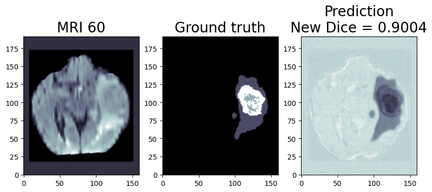
This application is available on the Intel® Developer Catalog for the developers to use as it is or use as a base code to bootstrap their customized solution. Intel® Developer Catalog offers reference implementations and software packages to build modular applications using containerized building blocks. Using the containerized building blocks the developers can rapidly develop deployable solutions.

Conclusion:

In conclusion, brain tumor segmentation using machine learning can help improve the accuracy and efficiency of the diagnosis and treatment of brain tumors.

There are several challenges and limitations to using machine learning for brain tumor segmentation. One of the main challenges is the limited availability of annotated data, as it is time consuming and expensive to annotate large datasets of medical images. In addition, there is a high degree of variability and complexity in the data, as brain tumors can have different shapes, sizes, and intensity patterns on MRI scans. This can make it difficult for the machine learning algorithm to generalize and accurately classify tumors in new data.

Another challenge is the potential for bias in the training data, as the dataset may not be representative of the entire population. This can lead to inaccurate or biased results if the algorithm is not properly trained or validated.

While there are still challenges to be overcome, the use of machine learning in medical image analysis shows great promise for improving patient care.

‍Notices & Disclaimers:

Intel technologies may require enabled hardware, software or service activation.

No product or component can be absolutely secure. 

Your costs and results may vary. 

© Intel Corporation. Intel, the Intel logo, and other Intel marks are trademarks of Intel Corporation or its subsidiaries.  Other names and brands may be claimed as the property of others.   

‍