
Hardware

OpenVINO is powered by OneDNN for the best performance on discrete GPU
OpenVINO and OneDNN
OpenVINO™ is a framework designed to accelerate deep-learning models from DL frameworks like Tensorflow or Pytorch. By using OpenVINO, developers can directly deploy inference application without reconstructing the model by low-level API. It consists of various components, and for running inference on a GPU, a key component is the highly optimized deep-learning kernels, such as convolution, pooling, or matrix multiplication.
On the other hand, Intel® oneAPI Deep Neural Network Library (oneDNN), is a library that provides basic deep-learning building blocks, mainly kernels. It differs from OpenVINO in a way that OneDNN provides APIs for running deep-learning nodes like convolution, but not for running deep-learning models such as Resnet-50.
OpenVINO utilizes OneDNN GPU kernels for discrete GPUs, in addition to its own GPU kernels. It is to accelerate compute-intensive workloads to an extreme level on discrete GPUs. While OpenVINO already includes highly-optimized and mature deep-learning kernels for integrated GPUs, discrete GPUs include a new hardware block called a systolic array, which accelerates compute-intensive kernels. OneDNN provides these kernels with systolic array usage.
If you want to learn more about the systolic array and the advancements in discrete GPUs, please refer to this article.
How does OneDNN accelerates DL workloads for OpenVINO?
When you load deep-learning models in OpenVINO, they go through multiple stages called graph compilation. The purpose of graph compilation is to create the "execution plan" for the model on the target hardware.
During graph compilation, OpenVINO GPU plugin checks the target hardware to determine whether it has a systolic array or not. If the hardware has a systolic array(which means you have a discrete GPU like Arc, Flex, or GPU Max series), OpenVINO compiles the model so that compute-intensive layers are processed using OneDNN kernels.
OpenVINO kernels and OneDNN kernels use a single OpenCL context and shared buffers, eliminating the overhead of buffer-copying. For example, OneDNN layer computes a layers and fills a buffer, which then may be read by OpenVINO kernels because both kernels run in a single OpenCL context.
You may wonder why only some of the layers are processed by OneDNN while others are still processed by OpenVINO kernels. This is due to the variety of required kernels. OneDNN includes only certain key kernels for deep learning while OpenVINO contains many kernels to cover a wide range of models.
OneDNN is statically linked to OpenVINO GPU Plugin, which is why you cannot find the OneDNN library from released OpenVINO binary. The dynamic library of OpenVINO GPU Plugin includes OneDNN.
The GPU plugin and the CPU plugin have separate versions of OneDNN. To reduce the compiled binary size, the OpenVINO GPU plugin contains only the GPU kernels of OneDNN, and the OpenVINO CPU plugin contains only the CPU kernels of OneDNN.
Hands-on Tips and FAQs
What should an application developer do to take advantage of OneDNN?
If the hardware supports a systolic array and the model has layers that can be accelerated by OneDNN, it will be accelerated automatically without any action required from application developers.
How can I determine whether OneDNN kernels are being used or not?
You can check the OneDNN verbose log or the executed kernel names.
Set `ONEDNN_VERBOSE=1` to see the OneDNN verbose log. Then you will see a bunch of OneDNN kernel execution log, which means that OneDNN kernels are properly executed. Each execution of OneDNN kernel will print a line. If all kernels are executed without OneDNN, you will not see any of such log line.
Alternatively, you can check the kernel names from performance counter option from benchmark_app. (--pc)
OneDNN layers include colon in the `execType` field as shown below. In this case, convolutions are handled by OneDNN jit:ir kernels. MaxPool is also handled by OneDNN kernel that is implemented with OpenCL.(and in this case, the systolic array is not used)
Can we run networks without Onednn on discrete GPU?
It is not supported out-of-box and it is not recommended to do so because systolic array will not be used and the performance will be very different.
If you want to try without OneDNN still, you can follow this documentation and use `OV_GPU_DisableOnednn`.
How to know whether my GPU will be accelerated with OneDNN(or it has systolic array or not)?
You can use hello_query_device from OpenVINO sample app to check whether it has `GPU_HW_MATMUL` in `OPTIMIZATION_CAPABILITIES`.
How to check the version of OneDNN?
You can set `ONEDNN_VERBOSE=1` to check see the verbose log. Below, you can see that OneDNN version is v3.1 as an example. (OnnDNN 3.1 was used for OpenVINO 23.0 release)
Please note that it is shown only when OneDNN is actually used in the target hardware. If the model is not accelerated through OneDNN, OneDNN version will not be shown.
Is it possible to try different OneDNN version?
As it is statically linked, you cannot try different OneDNN version from single OpenVINO version. It is also not recommended to build OpenVINO with different OneDNN version than it is originally built because we do not guarantee that it works properly.
How to profile OneDNN execution time?
Profiling is also integrated to OpenVINO. So you can use profiling feature of OpenVINO, such as --pc and --pcsort option from benchmark_app. However, it includes some additional overhead for OneDNN and it may report higher execution time than actual time especially for small layers. More reliable method is to use DevicePerformanceTiming with opencl-intercept-layers.
Deploy AI Workloads with OpenVINO™ Model Server across CPUs and GPUs
Authors: Xiake Sun, Kunda Xu
1. Introduction
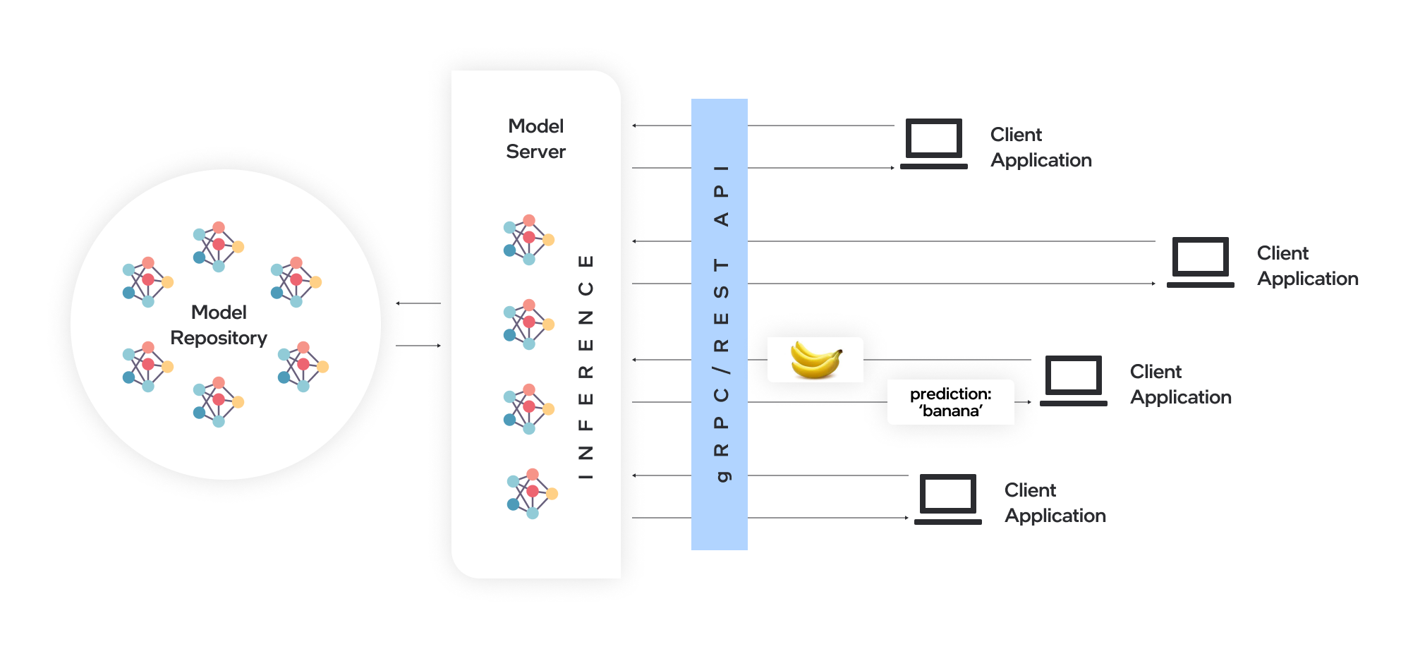
OpenVINO™ Model Server (OVMS) is a high-performance system for serving models. Implemented in C++ for scalability and optimized for deployment on Intel® architectures, the model server uses the same architecture and API as TensorFlow Serving and KServe while applying OpenVINO™ for inference execution. Inference service is provided via gRPC or REST API, making deploying new algorithms and AI experiments easy.
Docker is the recommended way to deploy OpenVINO™ Model Server. Pre-built container images are available on Docker Hub and Red Hat Ecosystem Catalog.
In this blog, we will introduce how to leverage OpenVINO™ Model Server to deploy AI workload across various hardware platforms, including Intel® CPU, Intel® GPU, and Nvidia GPU.
2. OpenVINO™ Model Server Pre-built Docker Image for Intel® CPU
Pull the latest pre-built OVMS docker image hosted in Docker Hub:
Verify OVMS docker image and OpenVINO™ backend version:
Here is an example output of the command line above:

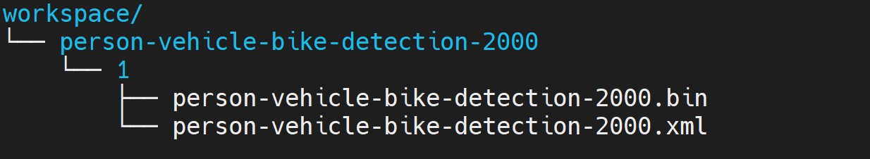
Download a model and create an appropriate directory structure. For example, a person-vehicle-bike-detection model from Intel’s Open Model Zoo:
where a model directory structure looks like that:
After the model repository preparation, let’s start OVMS to host a person-vehicle-bike-detection-2000 model in the Model Server with Intel® CPU as target device.
The parameter “--target_device CPU” specified workload to allocate on Intel® CPU. “--port 30001” set up the gRPC server port as 30001, and “--rest_port 30001” set up the REST server port as 30002. The parameter “--model_path” specified the model directory path in the docker image, while “--model_name” specified which model to host in the model server.
3. Build OpenVINO™ Model Server Benchmark Client
OpenVINO™ Model Server provides a useful tool - Benchmark Client to generate traffic and measure the performance of the model served in OpenVINO™ Model Server. In this blog, you could use Benchmark Client to verify OpenVINO™ model server functionality quickly.
To build the docker image and tag it as benchmark_client as follow:
Here is an example to use benchmark_client to generate 8 requests and send them via gRPC API, then receive the severed model performance data:
In the output, "window_netto_frame_rate" measures the overall performance of a service - how many frames per second the model server processed. Please note, model serving example above was set up with default parameters, see the performance tuning section for more details.
4. Build OpenVINO™ Model Server from Source Code
Download the model server source code as follows:
OVMS provides a “Makefile” to build the docker image with environment parameters, which you can pass via the command line for the building process.
- BASE_OS: base OS docker image used to build OVMS docker image, current supported values are “ubuntu” (by default) and “redhat”.
- OV_USE_BINARY: control whether to use a pre-built OpenVINO™ binary package for building OVMS docker image. If "OV_USE_BINARY=1", OVMS use a pre-built OpenVINO™ binary package. If "OV_USE_BINARY=0", OpenVINO™ will be built from source code during OVMS building process.
- DLDT_PACKAGE_URL: If "OV_USE_BINRAY=1", "DLDT_PACKAGE_URL" is used to set the URL path to the pre-built OpenVINO™ binary package
- GPU: control whether to enable OVMS support for Intel® GPU. By default, “GPU=0” disables OVMS support for Intel® GPU. If "GPU=1", OVMS support for intel® GPU will be enabled.
- NVIDIA: control whether to enable OVMS support for Nvidia GPU. By default, "NVIDIA=0" disables OVMS support for Nvidia GPU. If "NVIDIA=1", OVMS support for Nvidia GPU will be enabled, which requires building OpenVINO from the source code.
- OV_SOURCE_BRANCH: If "OV_USE_BINARY=0", "OV_SOURCE_BRANCH" is used to set the target branch or commit hash of OpenVINO source code. The default value is “master”
- OV_CONTRIB_BRANCH: If "NVIDIA=1", "OV_CONTRIB_BRANCH" is used to set the target branch or commit hash of OpenVINO contrib source code. The default value is “master"
Here is an example of building OVMS with the "releases/2022/3" branch of OpenVINO™ GitHub source code with target device Intel® CPU.
Built docker image will be available in the host as “openvino/model_server:latest”.
5. Build OpenVINO™ Model Server with Intel® GPU Support
Since OpenVINO™ 2022.3 release, OpenVINO™ added full support for Intel’s integrated GPU, Intel’s discrete graphics cards, such as Intel® Data Center GPU Flex Series, and Intel® Arc™ GPU for DL inferencing workloads in the intelligent cloud, edge, and media analytics workloads. OpenVINO™ Model Server 2022.3 also added support for Intel® GPU. The pre-built OpenVINO™ Model Server docker image with GPU driver for Intel® GPU is available in Docker Hub:
Here is an example of building OVMS with Intel® GPU support based on the OpenVINO™ source code:
The default GPU driver (version 22.8 for RedHat 8.7 or version 22.35 for Ubuntu 20.04) will be installed during the building process. Built docker image will be available in the host as “openvino/model_server:latest-gpu”.
Here is an example to launch the OVMS docker image with Intel® GPU as target device:
The parameter “--target_device GPU” specified workload to allocate on Intel® GPU. The parameter “--device /dev/dri” is used to pass the device context. The parameter “--group-add=$(stat -c"%g" /dev/dri/render\* | head -n 1) -u $(id -u):$(id -g)” is used to ensure the model server process security context account with correct permissions to run inference on Intel® GPU.
Here is an example to verify the severed model performance on Intel® GPU with benchmark_client:
6. Build OpenVINO™ Model Server with Nvidia GPU Support
OpenVINO™ Model Server can also support Nvidia GPU cards by using NVIDIA plugin from the GitHub repo openvino_contrib. Here is an example of building OVMS with Nvidia GPU support step by step:
First, pull the Nvidia docker base image with the GPU driver, e.g.,“docker.io/nvidia/cuda:11.8.0-runtime-ubuntu20.04”, please ensure to install same GPU driver version in the local host environment.
Install Nvidia Container Toolkit to expose the GPU driver to docker and restart docker.
Build OVMS docker image with Nvidia GPU support.“NVIDIA=1” enables to build OVMS with Nvidia GPU support, and “OV_USE_BINARY=0” enables building OpenVINO from the source code. Besides, “OV_SOURCE_BRANCH=releases/2022/3” refer to the OpenVINO™ GitHub "releases/2022/3" branch, while “OV_CONTRIB_BRANCH=releases/2022/3” refer to the OpenVINO contrib GitHub "releases/2022/3" branch.
Built docker image will be available in the host as “openvino/model_server-cuda:latest”.
Here is an example to launch the OVMS docker image with Nvidia GPU as target device:
The parameter “--target_device NVIDIA” is specified to allocate workload on NVIDIA GPU. The parameter “--gpu all” flag is used to access all GPU resources available in the host system.
Here is an example to verify the severed model performance on Nvidia GPU with benchmark_client:
7. Migration from Triton Inference Server to OpenVINO™ Model Server
KServe, as a robust and extensible cloud-native model server for Kubernetes, is widely adopted by model servers including Triton Inference Server. Since the 2022.3 release, OpenVINO™ Model Server added KServer API that supports REST and gRPC calls. Therefore, OVMS with Nvidia GPU support is fully compatible to receive requests from Triton Inference Client and run inference on Nvidia GPU.
Here is an example to pull the Triton Inference Server docker image:
Then you could use perf_client tools in the docker image to send generated workload as requests to OVMS via KServe API with gRPC port, then receive measured performance data on Nvidia GPU.
The simple example above shows how smoothly developers can migrate their own AI service workload from Triton Inference Server to OpenVINO™ Model Server without any change from the client.
Leverage the power of Model Caching in your AI Applications
Authors: Devang Aggarwal, Eddy Kim, Preetha Veeramalai
Choosing the right type of hardware for deep learning tasks is a critical step in the AI development workflow. Here at Intel, we provide developers, like yourself, with a variety of hardware options to meet your compute requirements. From Intel® CPUs to Intel® GPUs, there are a wide array of hardware platforms available to meet your needs. When it comes to inferencing on different hardware, the little things matter. For example, the loading of deep learning models, which can be a lengthy process and can lead to a difficult user experience on application startup.
Are there ways to achieve faster model loading time on such devices?
Short answer is, yes, there are ways; one way is to handle the model loading time. Model loading performs several time-consuming device-specific optimizations and network compilations, which can also result in developers seeing a relatively higher first inference latency. These delays can lead to a difficult user experience during application startup. This problem can be solved through a mechanism called Model Caching. Model Caching solves the issue of model loading time by caching the final optimized model directly into a file. Reusing cached networks can significantly reduce the model loading time.
Model Caching
With OpenVINO 2022.3, model caching is currently implemented as a preview feature. To accelerate first inference latency on Intel® GPU, not only should the kernel source code be compiled in a form that can be executed on the GPU, but also various optimization passes must be performed. Kernel caching reuses only the kernels, but model caching reuses even the output of the optimization passes, so the model loading time can be further reduced. Before model caching, kernel caching was used in the same manner: by setting the CACHE_DIR configuration key to a folder where the cache should be stored. Now, to use the preview feature of model caching, set the OV_GPU_CACHE_MODEL environment variable to 1. Since the extension of the cache file created by kernel caching is “cl_cache” and the extension of the cache file created by model caching is “blob”, it is possible to check whether model caching is activated through this.
Note: Currently this is a preview feature with OpenVINO 2022.3. This feature will be fully available in OpenVINO 2023.0.
Developers can now also leverage this preview feature from OpenVINO™ Toolkit in OpenVINO™ Execution Provider for ONNX Runtime, a product that accelerates inferencing of ONNX models using ONNX Runtime API’s while using the OpenVINO™ toolkit as a backend. With the OpenVINO™ Execution Provider, ONNX Runtime delivers better inferencing performance on the same hardware compared to generic acceleration on Intel® CPU, GPU, and VPU. Additionally, by using model caching, OpenVINO™ Execution Provider can speed up the first inference latency of deep learning models on Intel® GPU.
In OpenVINO™ Execution Provider for ONNX Runtime, the model caching feature can been abled by setting the ONNX Runtime config option ‘use_compiled_network’ to True while using the C++/Python API’s. This config option acts like a switch to enable and disable the model caching feature that saves the final optimized model into a .blob file during the very first inference of the model on Intel® hardware.
The blobs are loaded from a directory named ‘ov_compiled_blobs’ relative to the executable path by default. This path however can be overridden using the ONNX Runtime config option ‘blob_dump_path’ which is used to explicitly specify the path where you would like to dump and load the blobs files from when already using theuse_compiled_network (model caching) setting.
Refer to Configuration Options for more information about using these options.
Conclusion
With the Model Caching feature, the deep learning model loading time should significantly decrease. You can now utilize this feature in both the Intel® Distribution of OpenVINO™ Toolkit and OpenVINO™ Execution Provider for ONNX Runtime and experience better first inference latency for your AI models.
Notices & Disclaimers
Intel technologies may require enabled hardware, software or service activation.
No product or component can be absolutely secure.
Your costs and results may vary.
©Intel Corporation. Intel, the Intel logo, and other Intel marks are trademarks of Intel Corporation or itssubsidiaries. Other names and brands maybe claimed as the property of others.
Use Metrics to Scale Model Serving Deployments in Kubernetes
In this blog you will learn how to set up horizontal autoscaling in Kubernetes using inference performance metrics exposed by OpenVINO™ Model Server. This will enable efficient scaling of model serving pods for inference on Intel® CPUs and GPUs.
Why use custom metrics?
OpenVINO™ Model Server provides high performance AI inference on Intel CPUs and GPUs that can be scaled in Kubernetes. However, when it comes to automatic scaling in Kubernetes, the Horizontal Pod Autoscaler by default, relies on CPU utilization and memory usage metrics only. Although resource consumption indicates how busy the application is, it does not clearly say whether serving provides expected quality of service to the clients or not. Since OpenVINO Model Server exposes performance metrics, we can automatically scale based on service quality rather than resource utilization.
The first metric that comes to mind when thinking about service performance is the duration of request processing, otherwise known as latency. For example, mean or median over a specified period or latency percentiles. OpenVINO Model Server provides such metrics but setting autoscaling based on latency requires specific knowledge about each model and the environment where the inference is running in order to properly set thresholds that trigger scaling.
While autoscaling based on latency works and may be a good choice when you have model-specific knowledge, we will instead focus on a more generic metric using ovms_requests_streams_ratio. Let’s dive into what this means.
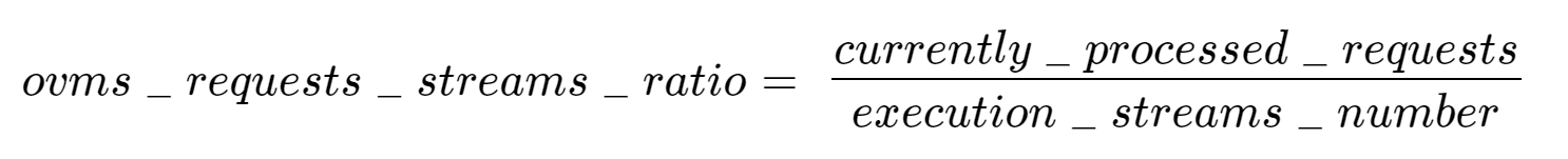
In the equation above:
- currently_processed_requests - number of inference requests to a model being processed by the service at a given time.
- execution_streams_number – number of execution streams. (When a model is loaded on the device, its computing units are divided into streams. Each stream independently handles inference requests, meaning that the number of streams defines how many inferences can be run on the device in parallel. Note that the more streams there are, the less powerful they are, so we get more throughput at a cost of higher minimal latency / inference time.)
In this equation, for any model exceeding a value of 1 indicates that requests are starting to queue up. Setting the autoscaler threshold for the ovms_requests_streams_ratio metric is somewhat of an arbitrary decision that should be made by a cluster administrator. Setting the threshold too low will result in underutilization of nodes and setting it too high will force the system to work with insufficient resources for extended periods of time. Now that we have chosen a metric for autoscaling, let’s start setting it up.
Deploy Model Server with Autoscaling Metrics
First, we need to create a deployment of OpenVINO Model Server in Kubernetes. To do this, follow instructions to install the OpenVINO Operator in your Kubernetes cluster. Then create a configuration where we can specify the model to be served and enable metrics:
Create ConfigMap:
With the configuration in place, we can deploy OpenVINO Model Server instance:
Create ModelServer resource:
Deploy and Configure Prometheus
Next, we need to read serving metrics and expose them to the Horizontal Pod Autoscaler. To do this we will deploy Prometheus to collect serving metrics and the Prometheus Adapter to expose them to the autoscaler.
Deploy Prometheus Monitoring Tool
Let’s start with Prometheus. In the example below we deploy a simple Prometheus instance via the Prometheus Operator. To deploy the Prometheus Operator, run the following command:
Next, we need to configure role-based access control to give Prometheus permission to access the Kubernetes API:
The last step is to create a Prometheus instance by deploying Prometheus resource:
If the deployment was successful, a Prometheus service should be running on port 9090. You can set up a port forward for this service, enabling access to the web interface via localhost on your machine:
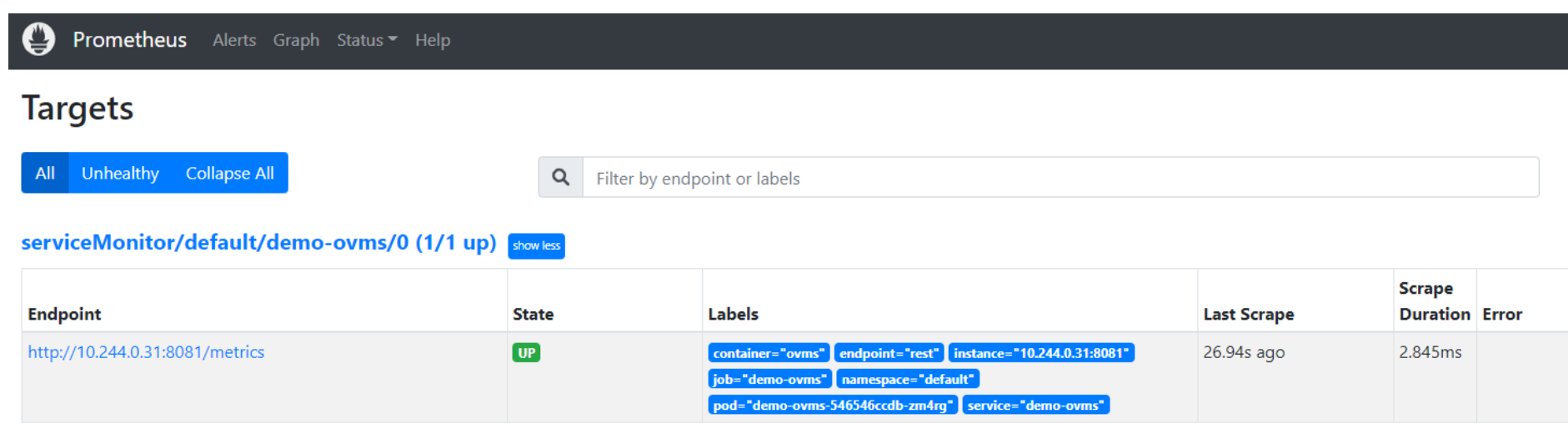
Now, when you open http://localhost:9090 in a browser you should see the Prometheus user interface. Next, we need to expose the Model Server to Prometheus by creating a ServiceMonitor resource:
Once it’s ready, you should see a demo-ovms target in the Prometheus UI:
Now that the metrics are available via Prometheus, we need to expose them to the Horizonal Pod Autoscaler. To do this, we deploy the Prometheus Adapter.
Deploy Prometheus Adapter
Prometheus Adapter can be quickly installed via helm or step-by-step via kubectl. For the sake of simplicity, we will use helm3. Before deploying the adapter, we will prepare a configuration that tells it how to expose the ovms_requests_streams_ratio metric:
Create a ConfigMap:
Now that we have a configuration, we can install the adapter:
Keep checking until custom metrics are available from the API:
Once you see the output above, you can configure the Horizontal Pod Autoscaler to use these metrics.
Set up Horizontal Pod Autoscaler
As mentioned previously, we will set up autoscaling based on the ovms_requests_streams_ratio metric and target an average value of 1. This will try to keep all streams busy all the time while preventing requests from queueing up. We will set minimum and maximum number of replicas to 1 and 3, respectively, and the stabilization window for both upscaling and downscaling to 120 seconds:
Create HorizontalPodAutoscaler:
Once deployed, you can generate some load for your model and see the results. Below you can see how Horizontal Pod Autoscaler scales the number of replicas by checking its status:

This data can also be visualized with a Grafana dashboard:
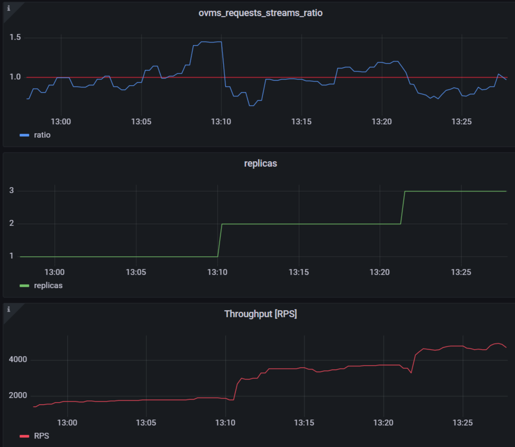
As you can see, with OpenVINO Model Server metrics, you can quickly set up inferencing system with monitoring and autoscaling for any model. Moreover, with custom metrics, you can set up autoscaling for inference on any Intel CPUs and GPUs.
See also:
- Load Balancing OpenVINO Model Server Deployments with Red Hat
- Kubernetes Device Plugin for Intel GPU
- OpenVINO Model Server metrics
Automatic Device Selection and Configuration with OpenVINO™
OpenVINO empowers developers to write deep learning application code once and deploy it on a wide range of Intel hardware with best-in-class performance. Previously, significant effort had to be spent configuring inference pipelines to squeeze optimal performance out of target hardware, and the effort had to be repeated whenever the application was ported to a new platform. The new Auto Device Plugin (AUTO) and automatic configuration features in OpenVINO make it easier for developers to unlock performance on multiple hardware targets without needing to spend time optimizing their application pipeline.
When an OpenVINO application is deployed in a system, the Auto Device Plugin automatically selects the best hardware target to inference the model with. OpenVINO then automatically configures the application to use optimal pipeline parameters based on the hardware capabilities and model size. Developers no longer need to write code for detecting hardware devices and explicitly configuring batch and stream parameters. High-level configuration is provided through performance hints that allow a developer to prioritize their application for either high throughput or minimal latency. AUTO and automatic device configuration make applications hardware-agnostic, allowing them to easily be ported to new hardware without any code changes.
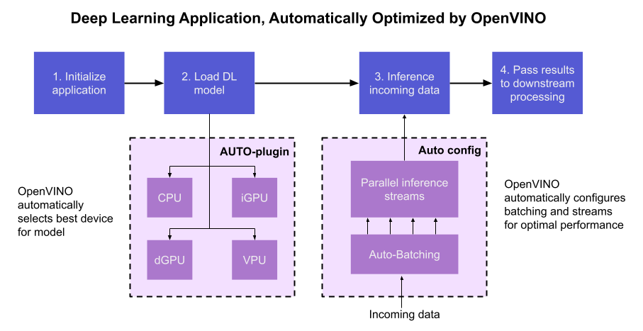
The diagram in Figure 1 shows how OpenVINO’s features automatically configure an application for optimal performance, regardless of the target hardware. When the deep learning model is loaded, AUTO creates a transparent plugin interface to the available processor devices and automatically selects the most suitable device. OpenVINO configures the batch size and number of processing streams based on the selected hardware target, and the Auto-Batching feature automatically groups incoming data into optimally sized batches. AUTO and automatic configuration operate independently from each other, so developers can use either or both in their application.
AUTO and automatic configuration are available starting in the 2022.1 release of OpenVINO Runtime. To use these features, simply install OpenVINO Runtime on the target hardware. The API uses AUTO by default if no processor device is specified when loading a model. Set a “throughput” or “latency” performance hint when loading the model, and the API automatically configures the inference pipeline. Read on to learn more about AUTO, automatic configuration, performance hints, and how to use them in your application.
Automatic Device Selection
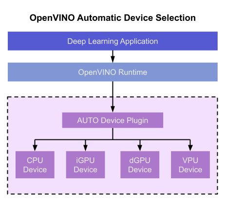
Auto Device Plugin (AUTO) is a “virtual” device that provides a transparent interface to physical devices in the system. When an application is initialized, AUTO discovers the available processors and accelerators in the system (CPUs, integrated GPUs, discrete GPUs, VPUs) and selects the best device, based on a default device priority list or an optional user-provided priority list. It creates an interface between the application and device that executes inference requests in an optimized fashion. It enables an application to always achieve optimal performance in a system without the developer having to know beforehand what devices are available in the system.
Key Features and Benefits
Simple and flexible application deployment
Previously, developers needed to know details about target hardware and configure their application specifically for each device. AUTO removes the need to write dedicated code for specific devices. This enables an application to be written once and deployed to any supported hardware. It also allows the application to run on newer generations of hardware as they are released: the developer only needs to compile the application with the latest version of OpenVINO to run it on new hardware. This provides an instant increase in performance with little development time.
Configurability
AUTO provides a configuration interface that is easy to use at a high level while still providing flexibility. Developers can simply specify “AUTO” as the device to tell the application to select the best device for the given model. They can also control which device is selected by providing a device candidate list and setting priorities for each device.
Developers can also use performance hints to configure their application for latency or throughput. When the performance hint is throughput, OpenVINO will create more streams for parallel inferencing to achieve maximum processing bandwidth. In latency mode, OpenVINO creates fewer streams to utilize as many resources as possible to complete each inference quickly. Performance hints also help determine the optimal batch size for inferencing; this is discussed further in the “Performance Hints” section of this document.
Improved first-inference latency
In applications that use accelerated processors like GPUs or VPUs, the time to first inference may be higher than average because it takes time to compile and load the deep learning model into the accelerator. AUTO solves this problem by starting the first inference with the CPU, which has minimal latency and no delays. As the first inference is being performed, AUTO continues to compile and load the model for the selected accelerator device, and then transparently switches over to that device when it is ready. This significantly reduces time to first inference, and is beneficial for applications that require immediate inference results on startup.
How Automatic Device Selection Works
To choose the best device for inference, AUTO discovers which hardware targets are available in the system and matches the model to the best supported device, using the following process:
- AUTO discovers which devices are available using the Query Device API. The query reads an internal file that lists installed hardware plugins, confirms the hardware modules are present by communicating with them through drivers, and returns a list of available devices in the system.
- AUTO checks the precision of the input model by reading the model file.
- AUTO selects the best available device in the device priority table (shown in Table 1 below) that is capable of supporting the model’s precision.
- AUTO attempts to compile the model on the selected device. If the model doesn’t compile (for example, if the device doesn’t support all the operations required by the model), AUTO tries to compile it on the next best device until compilation is successful. The CPU is the final fallback device, as it supports all operations and precisions.
By default, AUTO uses the device priority list shown in Table 1. Developers can customize the table to provide their own device priority list and limit the devices that are available to run inferencing. AUTO will not try to run inference on devices that are not provided in the device list.
Table 1. Default AUTO Device Priority List
As mentioned, AUTO reduces the first inference latency by compiling and loading the model to the CPU first. As the model is loaded to the CPU and first inference is performed, AUTO steps through the rest of the process for selecting the device and compiling the model to that device. This way, devices that require a long time for model compilation do not impede inference as the application is being initialized.
AUTO also provides a model priority feature that enables developers to control which models are loaded to which devices when there are multiple models running on a system with multiple devices. Developers can set “MODEL_PRIORITY” as “HIGH”, “MEDIUM”, or “LOW” to configure which models should be allocated to the best resource. This allows developers to ensure models that are critical for an application are always loaded to the fastest device for processing, while less critical models are loaded to slower devices.
For example, consider a medical imaging application with models for segmenting and/or classifying injuries in X-ray images running on a system that has both a GPU and a CPU. The segmentation model is set to HIGH priority because it takes more processing power to inference, while the classification model is set to MEDIUM priority. If both models are loaded at the same time, the segmentation model will be loaded to the GPU (the higher priority device) and the classification model will be loaded to the CPU (the lower priority device). If only the classification model is loaded, it will be loaded to the GPU since the GPU isn’t occupied by the higher-priority model.
Automatic Device Configuration
The performance of a deep learning application can be improved by configuring runtime parameters to fully utilize the target hardware. There are several factors to take into consideration when optimizing inference for a certain device, such as batch size and number of streams. (See Runtime Inference Optimizations in OpenVINO documentation for more information.) The optimal configuration for these parameters depends on the architecture and memory of the target hardware, and they need to be re-determined when porting an application from one device to another.
OpenVINO provides features that automatically configure an application to use optimal runtime parameters to achieve the best performance on any supported hardware target. These features are enabled through performance hints, which allow a user to specify whether their application should be optimized for latency or throughput. The automatic configuration eliminates the time and effort required to determine optimal configurations. It makes it simple to port to new devices or write one application to work on multiple devices. OpenVINO’s automatic configuration features currently work with CPU and GPU devices, and support for VPUs will be added in a future release.
Performance Hints
OpenVINO allows users to provide high-level "performance hints" for setting latency-focused or throughput-focused inference modes. These performance hints are “latency” and “throughput.” The hints cause the runtime to automatically adjust runtime parameters, such as number of processing streams and inference batch size, to prioritize for reduced latency or high throughput. Performance hints are supported by CPU and GPU devices, and a future release of OpenVINO will add support for VPUs.
The performance hints do not require any device-specific settings and are portable between devices. Parameters are automatically configured based on whichever device is being used. This allows users to easily port applications between hardware targets without having to re-determine the best runtime parameters for the new device.
Latency performance hint
Latency is the amount of time it takes to process a single inference request and is usually measured in milliseconds (ms). In applications where data needs to be inferenced and acted on as quickly as possible (such as autonomous driving), low latency is desirable. When applications are run with the “latency” performance hint, OpenVINO determines the optimal number of parallel inference requests for minimizing latency while still maximizing the parallelization capabilities of the hardware. It automatically sets the number of processing streams to achieve the best latency.
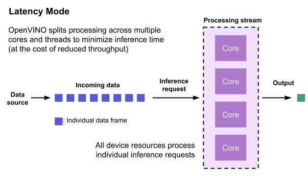
To achieve the fastest latency, the processor device should process only one inference request at a time so all the compute resources are available for calculation. However, devices with multiple cores (such as multi-socket CPUs or multi-tile GPUs) can deliver multiple streams with the same latency as they would with a single stream. OpenVINO automatically checks the compute demands of the model, queries capabilities of the device, and selects the number of streams to be the minimum required to get the best latency. For CPUs, this is typically one stream for each socket. For GPUs, it’s typically one stream per tile.
Throughput performance hint
Throughput is the amount of data an inferencing pipeline can process at once, and it is usually measured in frames per second (FPS) or inferences per second. In applications where large amounts of data needs to be inferenced simultaneously (such as multi-camera video streams), high throughput is needed. To achieve high throughput, the runtime should focus on fully saturating the device with enough data to process. When applications are run with the “throughput” performance hint, OpenVINO maximizes the number of parallel inference requests to utilize all the threads available on the device. On GPU, it automatically sets the inference batch size to fill up the GPU memory available.
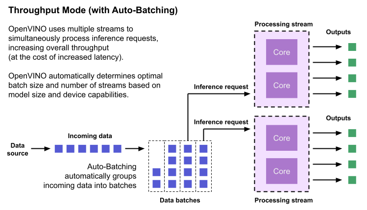
To configure the runtime for high throughput, OpenVINO automatically sets the number of streams to use based on the architecture of the device. For CPUs, it creates as many streams as there are cores available. For GPUs, it uses a combination of batch size and parallel streams to fully utilize the GPU’s memory and compute resources. To determine the optimal configuration on GPUs, OpenVINO will first check if the network supports batching. If it does, it loads the network with a batch size of one, determines how much memory is used for the single-batch network, and then scales the batch size and streams up to fill the entire GPU.
Batch size can also be explicitly specified in code when the model is loaded. This can be useful in applications where the number of incoming data sources is known and constant. For example, in an application that processes four camera streams, specify a batch size of four so that each set of frames from the cameras is processed in a single inference request. More information on batch configuration is given in the Auto-Batching section below.
Auto-Batching
Auto-Batching is a new feature of OpenVINO that performs on-the-fly grouping of data inference requests in an application. As the application makes individual inference requests, Auto-Batching transparently collects them into a batch. When the batch is full (or when a timeout limit is reached), OpenVINO executes inference on the whole batch. In short, it takes care of batching data efficiently so the developer doesn’t have to worry about it.
The Auto-Batching feature is controlled by the configuration parameter “ALLOW_AUTO_BATCHING”, which is enabled by default. Auto-Batching is activated when all of the following are true:
- ALLOW_AUTO_BATCHING is true
- The model is loaded to the target device with the throughput performance hint
- The target device supports batching (such as GPU)
- The model topology supports batching
When Auto-Batching is activated, OpenVINO automatically determines the optimal batch size for an application based on model size and hardware capabilities. Developers can also explicitly specify the batch size when loading the model. While the inference pipeline is active, individual inference requests are gathered into a batch and then executed when the batch is full.
Auto-Batching also has a timeout feature that is configurable by the developer. If there aren’t enough individual requests collected within the developer-specified time limit, batch execution will fall back to just using individual inference requests. For example, a developer may specify a timeout limit of 500 ms and a batch size of 16 for a video processing inference pipeline. Once 16 frames are gathered, a batch inference request is made. If only 13 frames arrive before the 500 ms timeout is hit, the application will perform individual inference requests on each of the 13 frames. While the timeout feature makes the pipeline robust to interruptions in incoming data, hitting the timeout limit heavily reduces the performance. To avoid this, developers should make sure there is enough incoming data to fill the batch within the time limit in typical conditions.
Auto-Batching, when combined with OpenVINO's automatic configuration features that determine optimal batch size and number of streams, provides a powerful benefit to the developer. The developer can utilize the full power of the target device with only using one line of code. Best of all, when an application is used on a different device, it will automatically reconfigure itself to achieve optimal performance with zero effort from the developer.
How to Use AUTO and Performance Hints
Using AUTO and automatic configuration with performance hints only requires one line of code. The functionality centers around the “ie.compile_model” method, which is used to compile a model and load it into device memory. The method accepts various configuration parameters that allow a user to provide high-level control over the pipeline.
Here are several Python examples showing how to configure a model and pipeline with the ie.compile_model method. The first example also shows how to import the OpenVINO Core model, initialize it, and read a model before calling ie.compile_model.
Example 1. Load a model on AUTO device
Example 2. Load a model on AUTO device with performance hints
Example 3. Provide a list of device candidates which AUTO may use when loading a model
Example 4. Load multiple models with HIGH, MEDIUM, and LOW priorities
Example 5. Load a model to GPU and use Auto-Batching with an explicitly set batch size
For a more in-depth example of how to use AUTO and automatic configuration, please visit the Automatic Device Selection with OpenVINO Jupyter notebook in the OpenVINO notebooks repository. It provides an end-to-end example that shows:
- How to download a model from Open Model Zoo and convert it to OpenVINO IR format with Model Optimizer
- How to load a model to AUTO device
- The improvement in first inference latency when using AUTO device
- How to perform asynchronous inferencing on data batches in throughput or latency mode
- A performance comparison between throughput and latency modes
The OpenVINO Benchmark App also serves as a useful tool for experimenting with devices and batching to see how performance changes under various configurations. The Benchmark App supports automatic device selection and performance hints for throughput or latency.
Where to Learn More
To learn more please visit auto device plugin and automatic configuration pages in OpenVINO documentation. They provide more information about how to use and configure them in an application.
OpenVINO also provides an example notebook explaining how to use AUTO and showing how it improves performance. The notebook can be downloaded and run on a development machine where OpenVINO Developer Tools have been installed. Visit the notebook at this link: Automatic Device Selection with OpenVINO.
To learn more about OpenVINO toolkit and how to use it to build optimized deep learning applications, visit the Get Started page. OpenVINO also provides a number of example notebooks showing how to use it for basic applications like object detection and speech recognition on the Tutorials page.
Accelerate Inference of Sparse Transformer Models with OpenVINO™ and 4th Gen Intel® Xeon® Scalable Processors
Authors: Alexander Kozlov, Vui Seng Chua, Yujie Pan, Rajesh Poornachandran, Sreekanth Yalachigere, Dmitry Gorokhov, Nilesh Jain, Ravi Iyer, Yury Gorbachev
Introduction
When it comes to the inference of overparametrized Deep Neural Networks, perhaps, weight pruning is one of the most popular and promising techniques that is used to reduce model footprint, decrease the memory throughput required for inference, and finally improve performance. Since Language Models (LMs) are highly overparametrized and contain lots of MatMul operations with weights it looks natural to prune the redundant weights and benefit from sparsity at inference time. There are several types of pruning methods available:
- Fine-grained pruning (single weights).
- Coarse pruning: group-level pruning (groups of weights), vector pruning (rows in weights matrices), and filter pruning (filters in ConvNets).
Contemporary Language Models are basically represented by Transformer-based architectures. Using coarse pruning methods for such models is problematic because of the many connections between the layers. This trait means that, first, not every pruning type is applicable to such models and, second, pruning of some dimension in one layer requires adjustments in the rest of the layers connected to it.
Fine-grained sparsity does not have such a constraint and can be applied to each layer independently. However, it requires special support on the HW and inference SW level to get real performance improvements from weight sparsity. There are two main approaches that help to leverage from weight sparsity at inference:
- Skip multiplication and addition for zero weights in dot products of weights and activations. This usually results in a special instruction set that implements such logic.
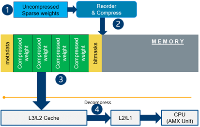
- Weights compression/decompression to reduce the memory throughput. Compression is performed at the model load/compilation stage while decompression happens on the fly right before the computation when weights are in the cache. Such a method can be implemented on the HW or SW level.
In this blog post, we focus on the SW weight decompression method and showcase the end-to-end workflow from model optimization to deployment with OpenVINO.
Sparsity support in OpenVINO
Starting from OpenVINO 2022.3release, OpenVINO runtime contains a feature that enables weights compression/decompression that can lead to performance improvement on the 4thGen Intel® Xeon® Scalable Processors. However, there are some prerequisites that should be considered to enable this feature during the model deployment:
- Currently, this feature is available only to MatMul operations with weights (Fully-connected layers). So currently, there is no support for sparse Convolutional layers or other operations.
- MatMul layers should contain a high level of weights sparsity, for example, 80% or higher which is achievable, especially for large Transformer models trained on simple tasks such as Text Classification.
- The deployment scenario should be memory-bound. For example, this prerequisite is applicable to cloud deployment when there are multiple containers running inference of the same model in parallel and competing for the same RAM and CPU resources.
The first two prerequisites assume that the model is pruned using special optimization methods designed to introduce sparsity in weight matrices. It is worth noting that pruning methods require model fine-tuning on the target dataset in order to reduce accuracy degradation caused by zeroing out weights within the model. It assumes the availability of the HW capable of DL model training. Nowadays, many frameworks and libraries offer such methods. For example, PyTorch provides some capabilities for NN pruning. There are also resources that offer pre-trained sparse models that can be used as a starting point, for example, SparseZoo from Neural Magic.
OpenVINO also provides instruments for DL model pruning implemented in Neural Network Compression Framework (NNCF) that is aimed specifically for model optimization and offers different optimization options: from post-training optimization to deep compression when stacking several optimization methods. NNCF is also integrated into Hugging Face Optimum library which is designed to optimize NLP models from Hugging Face Hub.
Using only sparsity is not so beneficial compared to another popular optimization method such as bit quantization which can guarantee better performance-accuracy trade-offs after optimization in the general case. However, the good thing about sparsity is that it can be stacked with 8-bit quantization so that the performance improvements of one method reinforce the optimization effect of another one leading to a higher cumulative speedup when applying both. Considering this, OpenVINO runtime provides an acceleration feature for sparse and 8-bit quantized models. The runtime flow is shown in the scheme below:
Below, we demonstrate two end-to-end workflows:
- Pruning and 8-bit quantization of the floating-point BERT model using Hugging Face Optimum and NNCF as an optimization backend.
- Quantization of sparse BERT model pruned with 3rd party optimization solution.
Both workflows end up with inference using OpenVINO API where we show how to turn on a runtime option that allows leveraging from sparse weights.
Pruning and 8-bit quantization with Hugging Face Optimum and NNCF
This flow assumes that there is a Transformer model coming from the Hugging Face Transformers library that is fine-tuned for a downstream task. In this example, we will consider the text classification problem, in particular the SST2 dataset from the GLUE benchmark, and the BERT-base model fine-tuned for it. To do the optimization, we used an Optimum-Intel library which contains the optimization capabilities based on the NNCF framework and is designed for inference with OpenVINO. You can find the exact characteristics and steps to reproduce the result in this model card on the Hugging Face Hub. The model is 80% sparse and 8-bit quantized.
To run a pre-optimized model you can use the following code from this notebook:
Quantization of already pruned model
In case if you deal with already pruned model, you can use Post-Training Quantization from the Optimum-Intel library to make it 8-bit quantized as well. The code snippet below shows how to quantize the sparse BERT model optimized for MNLI dataset using Neural Magic SW solution. This model is publicly available so that we download it using Optimum API and quantize on fly using calibration data from MNLI dataset. The code snippet below shows how to do that.
Enabling sparsity optimization inOpenVINO Runtime and 4th Gen Intel® Xeon® Scalable Processors
Once you get ready with the sparse quantized model you can use the latest advances of the OpenVINO runtime to speed up such models. The model compression feature is enabled in the runtime at the model compilation step using a special option called: “CPU_SPARSE_WEIGHTS_DECOMPRESSION_RATE”. Its value controls the minimum sparsity rate that MatMul operation should have to be optimized at inference time. This property is passed to the compile_model API as it is shown below:
An important note is that a high sparsity rate is required to see the performance benefit from this feature. And we note again that this feature is available only on the 4th Gen Intel® Xeon® Scalable Processors and it is basically for throughput-oriented scenarios. To simulate such a scenario, you can use the benchmark_app application supplied with OpenVINO distribution and limit the number of resources available for inference. Below we show the performance difference between the two runs sparsity optimization in the runtime:
- Benchmarking without sparsity optimization:
- Benchmarking when sparsity optimization is enabled:
Performance Results
We performed a benchmarking of our sparse and 8-bit quantized BERT model on 4th Gen Intel® Xeon® Scalable Processors with various settings. We ran two series of experiments where we vary the number of parallel threads and streams available for the asynchronous inference in the first experiments and we investigate how the sequence length impact the relative speedup in the second series of experiments.
The table below shows relative speedup for various combinations of number of streams and threads and at the fixed sequence length after enabling sparsity acceleration in the OpenVINO runtime.
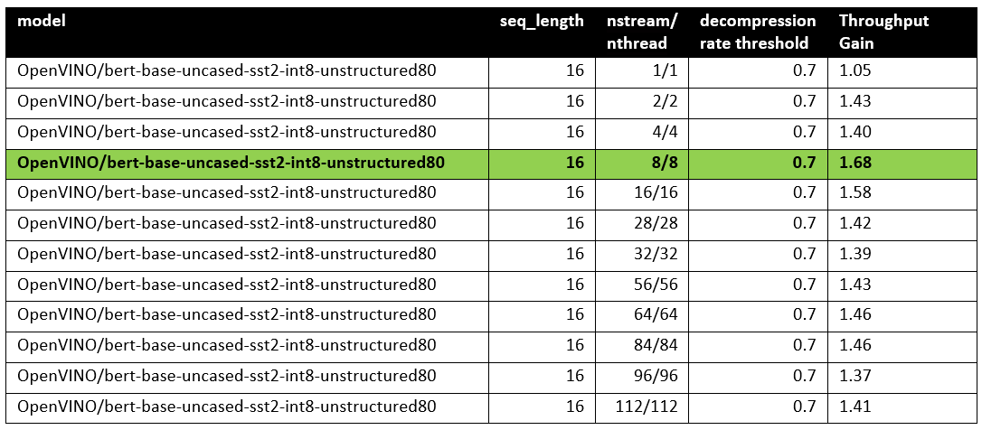
Based on this, we can conclude that one can expect significant performance improvement with any number of streams/threads larger than one. The optimal performance is achieved at eight streams/threads. However, we would like to note that this is model specific and depends on the model architecture and sparsity distribution.
The chart below also shows the relationship between the possible acceleration and the sequence length.
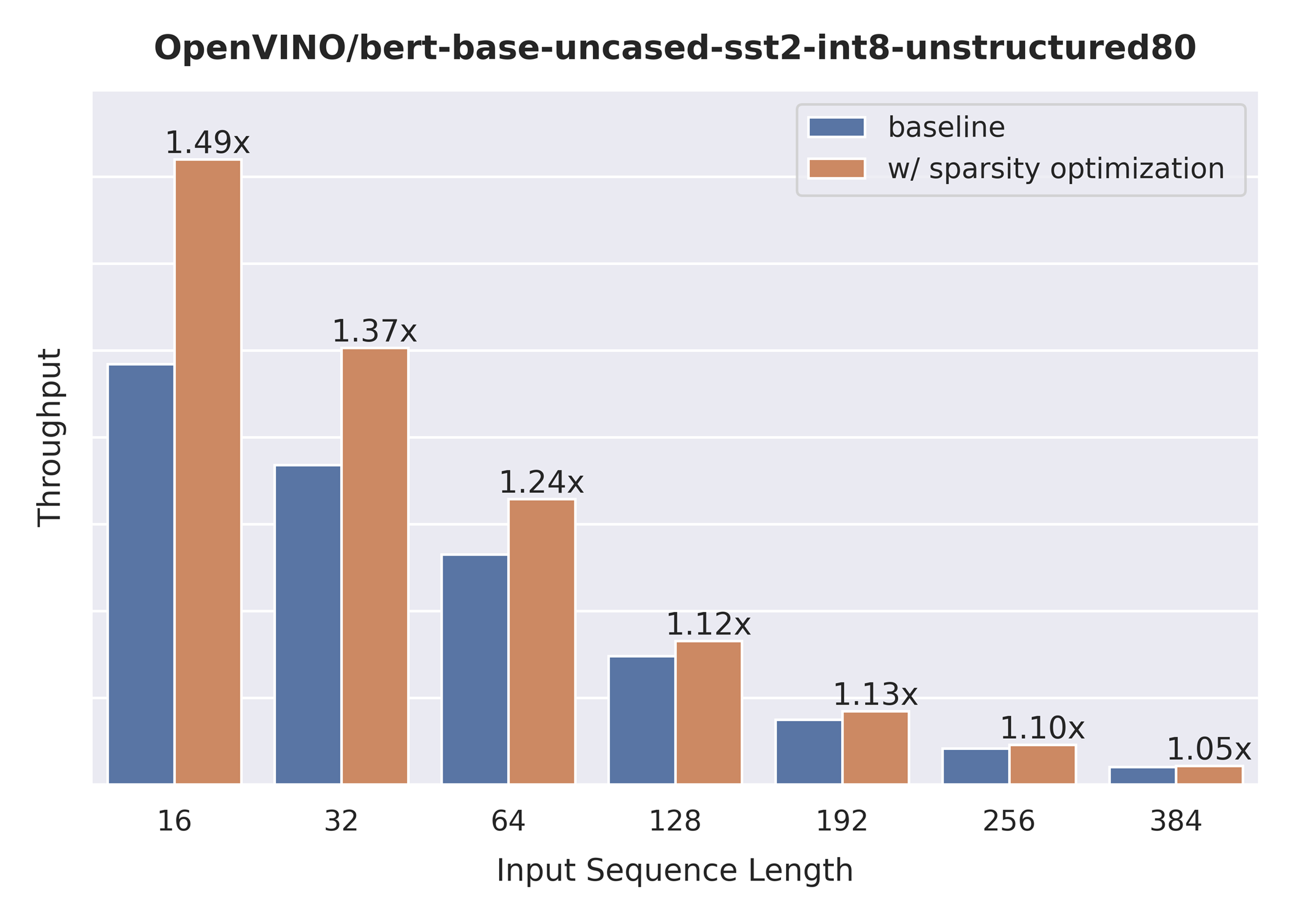
As you can see the benefit from sparsity is decreasing with the growth of the sequence length processed by the model. This effect can be explained by the fact that for larger sequence lengths the size of the weights is no longer a performance bottleneck and weight compression does not have so much impact on the inference time. It means that such a weight sparsity acceleration feature does not suit well for large text processing tasks but could be very helpful for Question Answering, Sequence Classification, and similar tasks.