

OpenVINO Blog

Q4'25: Technology Update – Low Precision and Inference Optimizations
Authors
Nikolay Lyalyushkin, Liubov Talamanova.
About
A quarterly digest on quantization, pruning, sparse attention, KV cache optimization, and related techniques for efficient AI inference.
Contributions welcome! We can't cover everything—if you spot something notable, open a PR in github.com/openvinotoolkit/technology_updates or let us know.
Summary
This quarter's research reveals several converging trends in efficient AI:
- Hadamard and learned rotations are now standard in quantization pipelines. The focus has shifted from whether to use rotations to how to compute them efficiently—via QR decomposition or per-block optimal transforms. New evidence shows integer formats (MXINT8, NVINT4) can outperform floating-point alternatives when combined with rotation-based outlier suppression.
- Diffusion-based video generation benefits from intelligent caching strategies with global outcome-aware metrics and principled optimization, replacing prior greedy approaches.
- LLM-based agents now achieve 100% correctness on KernelBench - GPU kernel benchmark.
Highlights
Quantization
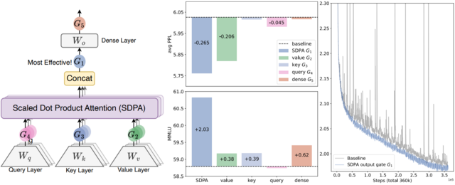
- Gated Attention for Large Language Models: Non-linearity, Sparsity, and Attention-Sink-Free (https://arxiv.org/pdf/2505.06708). The authors introduce Gated Attention, a simple architectural refinement that inserts a learnable, input-dependent sigmoid gate directly after the output of Scaled Dot-Product Attention, introducing query-dependent sparsity and crucial non-linearity between the value and final output projections. This minimal change suppresses redundant attention contributions, eliminates training instabilities like loss spikes, and consistently improves perplexity and downstream performance across both 15B MoE and 1.7B dense models trained on massive datasets. Notably, it directly addresses the root causes of the attention sink and massive activations through learned, input-sensitive sparsity—eliminating the need for manual workarounds like special sink tokens or ad hoc normalization tricks. As a result, the model exhibits far better long-context extrapolation, maintaining performance even when context lengths are extended beyond the training range. The reduction in extreme activation values and the elimination of disproportionate attention to early tokens suggest that this approach will make models more amenable to compression techniques such as quantization and token pruning, by creating a more uniform, sparse, and predictable activation profile. The code: https://github.com/qiuzh20/gated_attention
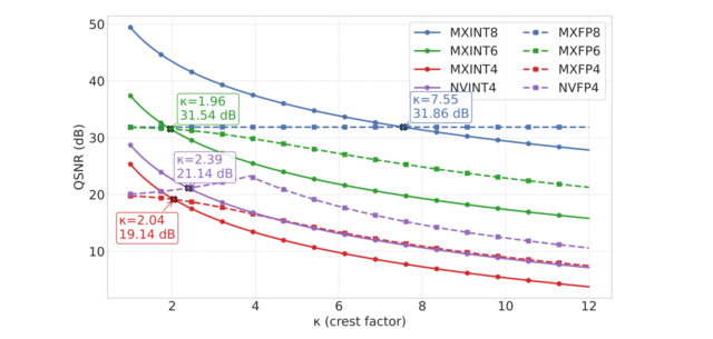
- INT v.s. FP: A Comprehensive Study of Fine-Grained Low-bit Quantization Formats (https://arxiv.org/abs/2510.25602). A comprehensive study on fine-grained, low-bit quantization formats challenges the current industry shift toward floating-point (FP) formats. The authors provide an in-depth analysis of quantization error using both theoretical Gaussian data and experimental training tensors, revealing a critical crossover point: floating-point formats are preferable for handling the high crest factors typical of coarse-grained quantization, whereas integer formats excel when crest factors are low, a condition common in fine-grained, block-wise quantization. Validating this insight across 12 diverse LLMs for direct-cast inference, the experiments consistently conclude that MXINT8 is superior to MXFP8 in accuracy and that NVINT4 can surpass NVFP4 when paired with outlier suppression techniques like Hadamard rotation. Furthermore, training experiments conducted with 1B and 3B Llama-3-style models demonstrate the superiority of MXINT8 over MXFP8, achieving nearly the same average accuracy across six common-sense reasoning tasks as standard BF16 training. The code: https://github.com/ChenMnZ/INT_vs_FP
Pruning / Sparsity
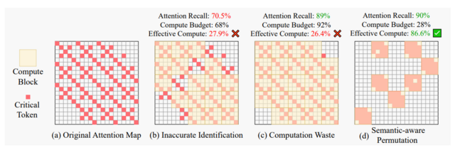
- Sparse VideoGen2: Accelerate Video Generation with Sparse Attention via Semantic-Aware Permutation (https://arxiv.org/pdf/2505.18875). SVG2 is a training-free sparse attention method designed to accelerate video generation in DiT-based models. Its core idea is to use semantic-aware permutation to better identify critical tokens and reduce unnecessary sparse-attention overhead. The method introduces three key techniques:
- Semantic-aware permutation: k-means clustering is applied to the Q/K/V vectors of each head and layer, and tokens are permuted by cluster to form semantically coherent blocks, improving the accuracy of critical-token detection.
- Dynamic top-p critical-token selection: Cluster centroids approximate attention scores, and clusters (and their tokens) are selected until the cumulative probability reaches p, enabling dynamic compute budgeting.
- Customized sparse-attention kernels: Since semantic-aware clusters vary naturally in size, custom kernels are used to support dynamic block sizes, which fixed-size sparse kernels cannot handle efficiently.
Notable results
Quantization
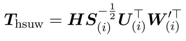
- WUSH: Near-Optimal Adaptive Transforms for LLM Quantization (https://arxiv.org/pdf/2512.00956). This work introduces WUSH, a method that derives optimal blockwise transforms for joint weight-activation quantization in large language models. WUSH consistently reduces quantization loss and improves LLM accuracy across MXFP4 and NVFP4 formats compared to the Hadamard transform across various LLM architectures (e.g., Llama-3.2-3B, Qwen3-14B). This comes at the cost of increased inference overhead, since WUSH computes a unique, data-dependent transform for each block, rather than reusing a single fixed Hadamard transform across all blocks.
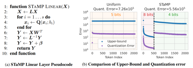
- STaMP: Sequence Transformation and Mixed Precision for Low-Precision Activation Quantization (https://arxiv.org/abs/2510.26771). STaMP is a post-training quantization technique designed to enhance the accuracy of low-bit activation quantization in large generative models by exploiting correlations along the sequence dimension rather than just the feature dimension. It combines invertible linear transformations—such as the Discrete Wavelet Transform (DWT) or Discrete Cosine Transform (DCT)—with mixed-precision quantization to concentrate the majority of activation energy into a small subset of tokens. These high-energy tokens are preserved at higher bit depths (e.g., 8-bit), while the remaining tokens are quantized to lower precision (e.g., 4-bit). The approach reduces quantization error more effectively than uniform bit allocation, especially under aggressive 4-bit constraints, and works synergistically with existing methods like SmoothQuant or QuaRot that operate on feature axes. Crucially, because the sequence transformation is orthogonal and linear, its inverse can often be merged with downstream operations such as bias addition or matrix multiplication, resulting in negligible additional computational cost during inference. The method requires no retraining and has been shown to improve both language and vision models consistently across benchmarks.
- KVLinC: KV CACHE QUANTIZATION WITH HADAMARD ROTATION AND LINEAR CORRECTION (https://arxiv.org/pdf/2510.05373v1). KVLinC is a framework designed to mitigate attention errors arising from KV cache quantization. The authors integrate two complementary techniques to enable robust low-precision caching. First, through a detailed analysis of Hadamard rotation-based quantization strategies, they show that applying channel-wise quantization to raw keys and token-wise quantization to Hadamard-transformed values minimizes quantization error. Second, to address residual errors from quantized keys, they propose lightweight linear correction adapters that explicitly learn to compensate for distortions in attention. Extensive evaluation across the Llama, Qwen2.5, and Qwen3 model families demonstrates that KVLinC consistently matches or surpasses strong baselines under aggressive KV-cache compression. Finally, the authors develop a custom attention kernel that delivers up to 2.55× speedup over FlashAttention, enabling scalable, efficient, and long-context LLM inference.
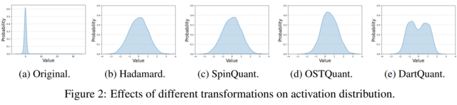
- DartQuant: Efficient Rotational Distribution Calibration for LLM Quantization(https://arxiv.org/pdf/2511.04063). DartQuant introduces an efficient method for quantizing large language models (LLMs). Instead of relying on computationally expensive end-to-end fine-tuning of rotation matrices—as done in methods like SpinQuant and OSTQuant—DartQuant eliminates the need for task-specific losses and instead optimizes activation distributions to be more uniform, using a novel loss function called Whip loss. This approach reduces the impact of extreme outliers in activations, which are a major source of quantization error, by reshaping the distribution from a Laplacian-like form toward a uniform one within a bounded range. To further reduce overhead, DartQuant proposes QR-Orth, an optimization scheme that leverages QR decomposition to enforce orthogonality on rotation matrices without requiring complex manifold optimizers like Cayley SGD. This cuts the computational cost of rotation calibration by 47× and memory usage by 10× on a 70B model, enabling full rotational calibration on a single consumer-grade RTX 3090 GPU in under 3 hours. The method maintains or slightly improves upon state-of-the-art quantization accuracy across multiple LLMs (Llama-2, Llama-3, Mixtral, DeepSeek-MoE) and evaluation benchmarks, including zero-shot reasoning tasks and perplexity metrics, while being robust to different calibration datasets and sample sizes. The code: https://github.com/CAS-CLab/DartQuant
Pruning / Sparsity
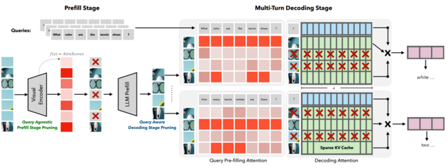
- SparseVILA: Decoupling Visual Sparsity for Efficient VLM Inference (https://arxiv.org/pdf/2510.17777). SparseVILA addresses the scalability limitations of Vision Language Models (VLMs) caused by the high computational cost of processing extensive visual tokens in long-context tasks. The framework introduces a decoupled sparsity paradigm that applies distinct optimization strategies to the prefill and decoding stages of inference. During the prefill phase, the model employs query-agnostic pruning to remove redundant visual data based on salience, efficiently creating a compact shared context. In contrast, the decoding phase utilizes query-aware retrieval to dynamically select only the specific visual tokens relevant to the current text query from the cache. This design preserves the integrity of multi-turn conversations by retaining a comprehensive visual cache, allowing different tokens to be retrieved for subsequent questions without permanent information loss. Experimental results demonstrate that SparseVILA achieves up to 2.6x end-to-end speedups on long-context video tasks while maintaining or improving accuracy across various image and reasoning benchmarks.
- THINKV: THOUGHT-ADAPTIVE KV CACHE COMPRESSION FOR EFFICIENT REASONING MODELS (https://arxiv.org/pdf/2510.01290v1). ThinKV is a KV cache compression framework for Large Reasoning Models (LRMs) on tasks like coding and mathematics. It classifies CoT tokens into Reasoning (R), Execution (E), and Transition (T) based on attention sparsity (T > R > E) using an offline calibration phase with Kernel Density Estimation to determine sparsity thresholds. The framework employs two main strategies:
- Think Before You Quantize: assigns token precision by importance. R/E tokens use 4-bit NVFP4, T tokens use 2-bit ternary, with group quantization (g=16) and shared FP8 (E4M3) scales; keys are quantized per-channel, values per-token. Outlier Transition thoughts are recognized as vital for backtracking and preventing model loops. Token importance is measured via KL divergence of the final answer distribution when a thought segment is removed.
- Think Before You Evict: a thought-adaptive eviction scheme aligned with PagedAttention. K-means clustering on post-RoPE key embeddings retains cluster centroids and corresponding values for evicted segments.

Caching
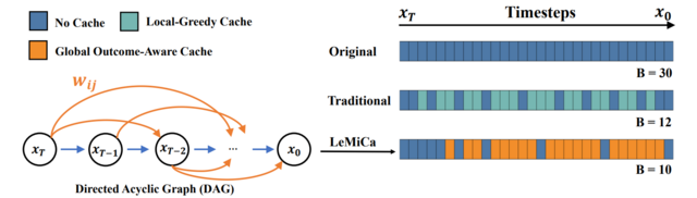
- LeMiCa: Lexicographic Minimax Path Caching for Efficient Diffusion-Based Video Generation (https://arxiv.org/pdf/2511.00090). LeMiCa is a novel, training-free, and efficient acceleration framework for diffusion-based video generation. The key idea is to take a global view of caching error using a Global Outcome-Aware error metric, which measures the impact of each cache segment on the final output. This approach removes temporal heterogeneity and mitigates error propagation. Using this metric, LeMiCa builds a Directed Acyclic Graph (DAG) in which each edge represents a potential cache segment, weighted by its global impact on output quality. The DAG is generated offline using multiple prompts and full sampling trajectories. LeMiCa then applies lexicographic minimax optimization to choose the path that minimizes worst-case degradation. Among all feasible paths under a fixed computational budget, it selects the one with the smallest maximum error. LeMiCa-slow achieves the highest reconstruction quality, reducing LPIPS from 0.134 → 0.05 on Open-Sora and 0.195 → 0.091 on Latte—over 2× improvement compared to TeaCache-slow. LeMiCa-fast improves inference speed from 2.60× → 2.93× on Latte relative to TeaCache-fast, while preserving visual quality. Unlike prior work that relies on online greedy strategies, LeMiCa precomputes its caching policy, eliminating runtime overhead. Code: https://unicomai.github.io/LeMiCa.
- CacheDiT: A PyTorch-native and Flexible Inference Engine with Hybrid Cache Acceleration and Parallelism for 🤗 DiTs (https://github.com/vipshop/cache-dit). It provides a unified cache API that supports features like automatic block adapters, DBCache, and more, covering almost all Diffusers' DiT-based pipelines. DBCache is a training-free Dual Block Caching mechanism inspired by the U-Net architecture. It splits the DiT Transformer block stack into three functional segments:
- Probe (front): performs full computation to capture residual signals and compare them with the previous step.
- Cache (middle): skips computation and reuses cached outputs when residual changes stay below a configurable threshold.
- Corrector (rear): always recomputes to refine outputs and correct any accumulated deviations. This probe → decision → correction loop enables structured, reliable caching that can be applied across DiT models without any retraining.
Inference
- vLLM-Gaudi - First Production-Ready vLLM Plugin for Intel® Gaudi® (https://docs.vllm.ai/projects/gaudi/en/v0.11.2/). Fully aligned with upstream vLLM, it enables efficient, high-performance large language model (LLM) inference on Intel® Gaudi®.
Compilation
- KernelFalcon: Autonomous GPU Kernel Generation via Deep Agents (https://pytorch.org/blog/kernelfalcon-autonomous-gpu-kernel-generation-via-deep-agents/). A deep agent architecture for generating GPU kernels that combines hierarchical task decomposition and delegation, a deterministic control plane with early-win parallel search, grounded tool use, and persistent memory/observability. KernelFalcon is the first known open agentic system to achieve 100% correctness across all 250 L1/L2/L3 KernelBench tasks.
Q3'25: Technology Update – Low Precision and Model Optimization
Authors
Nikolay Lyalyushkin, Liubov Talamanova, Alexander Suslov, Souvikk Kundu, Andrey Anufriev.
Summary
During Q3 2025, substantial progress was made across several fronts in efficient LLM inference — particularly in low-precision weight quantization, KV-cache eviction and compression, attention reduction through sparse and hybrid architectures, and architecture-aware optimization for State Space Models and Mixture-of-Experts. Notably, compression methods began to see adoption for FP4 formats, extending beyond traditional integer quantization, and numerous studies show that advanced KV-cache optimizations push the state of the art, achieving order-of-magnitude memory savings and notable speedups.
Highlights
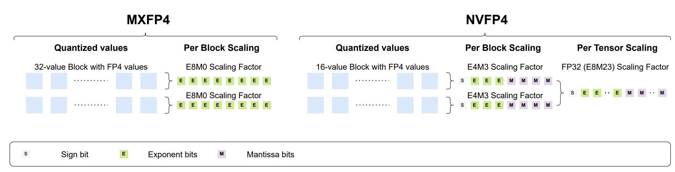
- Bridging the Gap Between Promise and Performance for Microscaling FP4 Quantization (https://arxiv.org/pdf/2509.23202). The authors provide a rigorous analysis of FP4 microscaling formats (MXFP4 and NVFP4) for LLM quantization, introduce Micro-Rotated-GPTQ (MR-GPTQ) and the QuTLASS GPU kernels to bridge the performance gap for such formats. The method uses MSE-optimized grids, static activation reordering, and fused online Hadamard rotations to recover 98-99% of FP16 accuracy while achieving up to 4x inference speedups on modern GPUs. Key insights from the analysis include:
- The effectiveness of Hadamard transforms depends on the quantization group size; while they are beneficial for MXFP4 and INT4, they can actually degrade NVFP4 accuracy.
- MR-GPTQ consistently improves the accuracy of the lower-performing MXFP4 format, bringing it within 1-2% of NVFP4's performance.
- On average, NVFP4 and INT4 (with group size 32) offer similar quality.
- MXFP4 kernels may achieve ~15% higher throughput than NVFP4 on B200 GPUs, likely due to simpler hardware implementation.
The code available at: https://github.com/IST-DASLab/FP-Quant.
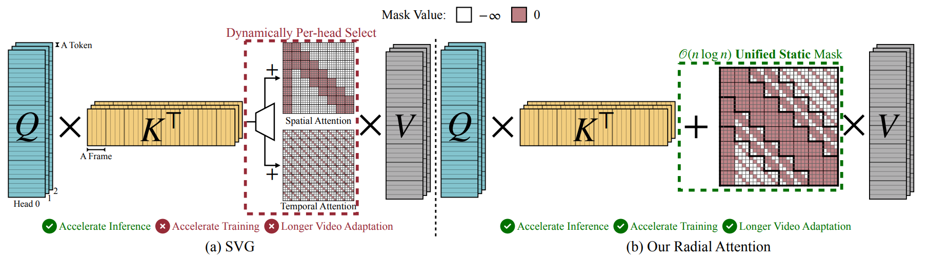
- Radial Attention: O(n log n) Sparse Attention with Energy Decay for Long Video Generation (https://arxiv.org/pdf/2506.19852). The paper "Radial Attention" introduces a sparse attention mechanism to optimize long video generation. Its core method reduces computational complexity from O(n2) to O(nlogn) using a static mask inspired by "Spatiotemporal Energy Decay," where attention focuses on spatially and temporally closer tokens. This architecture is highly optimized for inference. It delivers up to a 3.7x speedup on extended-length videos compared to standard dense attention, without any discernible loss in visual quality. For a concrete 500-frame, 720p video, the mechanism slashes the raw attention computation by a factor of 9x. The industrial impact is significant. Designed as a "plug-and-play" module, Radial Attention can be integrated into powerful pre-trained models like Wan2.1-14B and HunyuanVideo through efficient LoRA-based fine-tuning.
- Expected Attention: KV Cache Compression by Estimating Attention from Future Queries Distribution (https://arxiv.org/pdf/2510.00636). Expected Attention is a training-free KV cache compression method for LLMs that does not rely on observed attention scores, making it compatible with FlashAttention, where attention matrices are never materialized. It estimates the importance of cached key–value pairs by predicting how future queries will attend to them. Since hidden states before attention and MLP layers are empirically Gaussian-like, the method can analytically compute expected attention scores for each KV pair and rank them by importance for pruning. During decoding, Expected Attention maintains a small buffer of 128 hidden states to estimate future query statistics and performs compression every 512 generation steps. On LLaMA-3.1-8B, it achieves substantial memory savings—up to 15 GB reduction for 120k-token contexts. At a 50% compression ratio, Expected Attention maintains near-identical performance to the uncompressed baseline, effectively halving KV cache size while preserving output quality. Code: https://github.com/NVIDIA/kvpress
-
Papers with notable results
Quantization
- SINQ: Sinkhorn-Normalized Quantization for Calibration-Free Low-Precision LLM Weights (https://arxiv.org/pdf/2509.22944). The authors introduce a novel data-free post-training quantization method - SINQ. Instead of the traditional single-scale approach, SINQ employs dual scales: one for rows and another for columns. The method adapts the Sinkhorn-Knopp algorithm to normalize the standard deviations of matrix rows and columns. The algorithm is lightweight - operates at only 1.1x the runtime of basic RTN. The method proves robust across model scales, from small 0.6B parameter models to massive 235B parameter Mixture-of-Experts architectures. SINQ demonstrates orthogonality to other quantization advances. When combined with non-uniform quantization levels (NF4) or activation-aware calibration (A-SINQ with AWQ), it provides additional improvements.

- 70% Size, 100% Accuracy: Lossless LLM Compression for Efficient GPU Inference via Dynamic-Length Float (https://arxiv.org/pdf/2504.11651). The paper presents DFloat11, a dynamic-length float encoding scheme that exploits the low entropy of BFloat16 weights in large language models to achieve ~30% storage savings (reducing from 100% to ~70% size) without any loss in accuracy (bit-for-bit identical outputs). They do this by frequency-based variable-length coding of weight values, and couple it with a custom GPU decompression kernel allowing efficient inference. Experiments on large LLMs show major throughput gains and extended context length under fixed GPU memory budgets, making deployment more practical on resource-constrained hardware.
- XQUANT: Breaking the Memory Wall for LLM Inference with KV Cache Rematerialization (https://arxiv.org/pdf/2508.10395). This paper introduces XQuant, a memory-efficient LLM inference method that quantizes and caches input activations (X) of each transformer layer instead of Key-Value pairs. During inference, K and V are rematerialized on-the-fly by multiplying the cached X with the projection matrices, halving the memory footprint compared to standard KV caching. XQuant uses uniform low-bit quantization for X, which is more robust to aggressive quantization than K/V, enabling high compression with minimal accuracy loss. Building on this, XQuant-CL exploits cross-layer similarity in X embeddings by compressing the differences between successive layers, which have a smaller dynamic range due to the transformer's residual stream. Both XQuant and XQuant-CL outperform state-of-the-art KV cache quantization methods like KVQuant, while retaining accuracy close to the FP16 baseline. For GQA models, X is down-projected via offline SVD into a smaller latent space, preserving memory efficiency and accuracy. On LLaMA-2-7B and LLaMA-2-13B, XQuant achieves 7.7× memory savings with <0.1 perplexity degradation, while XQuant-CL reaches 12.5× savings at 2-bit precision (0.1 perplexity degradation) and 10× savings at 3-bit precision (0.01 perplexity degradation).
- Quamba2: A Robust and Scalable Post-training Quantization Framework for Selective State Space Models (https://arxiv.org/pdf/2503.22879). State Space Models (SSMs) are highly sensitive to quantization due to their linear recurrence process, which magnifies even minor numerical perturbations, making traditional Transformer quantization methods ineffective. The authors identify several distinctive properties of SSMs: (1) the input and output channel orders remain consistent, and (2) the activated channels and states are stable across time steps and input variations. Leveraging these insights, they propose Quamba2, a post-training quantization framework specifically tailored for SSMs. Quamba2 utilizes these properties through three key strategies: an offline sort-and-cluster process for input quantization, per-state-group quantization for input-dependent parameters, and cluster-aware weight reordering. The approach supports multiple precision configurations—W8A8, W4A8, and W4A16—across both Mamba1 and Mamba2 architectures. Empirical results show that Quamba2 surpasses existing SSM quantization methods on zero-shot and MMLU benchmarks. It achieves up to 1.3× faster pre-filling, 3× faster generation, and 4× lower memory usage on models such as Mamba2-8B, with only a 1.6% average accuracy drop. Code is available at https://github.com/enyac-group/Quamba.

- Qronos: Correcting the Past by Shaping the Future... in Post-Training Quantization (https://arxiv.org/pdf/2505.11695). The paper introduces Qronos, a new state-of-the-art post-training quantization (PTQ) algorithm for compressing LLMs. Its core innovation is that it unifies two critical error-handling strategies for the first time: it corrects for the "inherited" error propagated from previous layers and the "local" error from weights quantization within the current layer. This dual approach yields state-of-the-art results for small LLMs like Llama3-1B/3B/8B models. It can serve as a drop-in replacement for existing methods like GPTQ, running efficiently on resource-constrained hardware like AI laptops.

- Quantization Hurts Reasoning? An Empirical Study on Quantized Reasoning Models (https://arxiv.org/pdf/2504.04823). This paper conducts a systematic study on quantized reasoning models, evaluating the open-sourced DeepSeek-R1-Distilled Qwen and LLaMA families ranging from 1.5B to 70B params, QwQ-32B, and Qwen3-8B. The authors conducted quantization for weights, KV cache, and activation tensors. They claim that W8A8 or W4A16 may be treated as a form of lossless quantization. Specifically, for weights with 8-bit nearly all the quantization types generally lead to lossless accuracy, with no clear leading algorithm. While at 4-bit, FlatQuant emerges as a preferred algorithm and can yield near-lossless performance for the weight-only quantization scenario. For KV cache, the authors suggested 4-bit quantization as a safer choice, as at lower precision the models suffer from significant accuracy drop. Additionally, the authors claim that quantization may make more critical tasks more prone to error, with extreme low-precision models often generating longer sequences, hinting at longer thinking scenario. The code is available at: https://github.com/ruikangliu/Quantized-Reasoning-Models.
Pruning/Sparsity
- PagedEviction: Structured Block-wise KV Cache Pruning for Efficient Large Language Model Inference (https://arxiv.org/pdf/2509.04377). The authors propose PagedEviction, a structured block-wise KV cache eviction strategy designed for vLLM’s PagedAttention to enhance memory efficiency during large language model inference. The method computes token importance using the ratio of the L2 norm of Value to Key tokens, avoiding the need to store attention weights for compatibility with FlashAttention. It evicts an entire block only when the current block becomes full, reducing fragmentation and minimizing per-step eviction overhead. PagedEviction achieves high compression efficiency with minimal accuracy loss, significantly outperforming prior methods on long-context tasks. For example, it improves ROUGE scores by 15–20% over StreamingLLM and KeyDiff at tight cache budgets while closely matching full-cache performance at larger budgets across LLaMA-3.2-1B-Instruct and 3B-Instruct models.
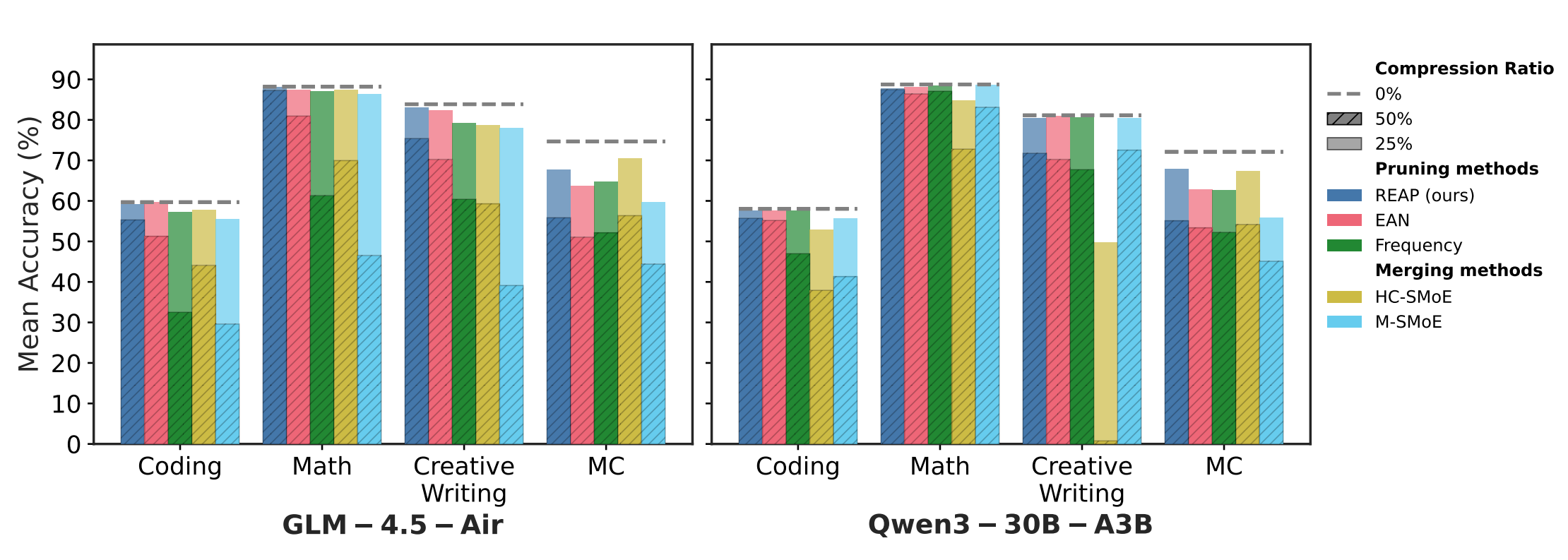
- REAP: One-Shot Pruning for Trillion-Parameter Mixture-of-Experts Models (https://arxiv.org/pdf/2510.13999). The authors show that merging experts introduces an irreducible error and substantially reduces the functional output space of the compressed SMoE layer. Leveraging this insight, they propose Router-weighted Expert Activation Pruning (REAP), a one-shot pruning method that removes low-impact experts while preserving model quality. REAP assigns each expert a saliency score that combines its router gate-values with its average activation norm, effectively identifying experts that are rarely selected and have minimal influence on the model’s output. Across sparse MoE architectures from 20B to 1T parameters, REAP consistently outperforms prior pruning and merging methods, particularly at 50% compression. It achieves near-lossless compression on code generation tasks, retaining performance after pruning 50% of experts from Qwen3-Coder-480B and Kimi-K2. Code is available at: https://github.com/CerebrasResearch/reap.
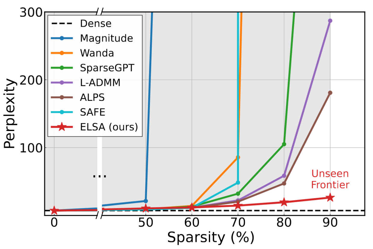
- The Unseen Frontier: Pushing the Limits of LLM Sparsity with Surrogate-Free ADMM (https://arxiv.org/pdf/2510.01650). This paper tackles the limitation of existing pruning methods for large language models, which struggle to exceed 50–60% sparsity without severe performance loss. The authors attribute this to the use of indirect objectives, such as minimizing layer-wise reconstruction errors, which accumulate mistakes and lead to suboptimal outcomes. To address this, the proposed method, ELSA, directly optimizes the true task objective — minimizing loss on actual downstream tasks — rather than relying on surrogate goals. It leverages the ADMM framework, a proven mathematical technique that decomposes complex problems into simpler alternating steps, to guide the pruning process while maintaining alignment with the model’s real objectives. A lightweight variant, ELSA-L, further improves scalability by using lower-precision data formats, enabling efficient pruning of even larger models. ELSA achieves 7.8× lower perplexity than the best existing method on LLaMA-2-7B at 90% sparsity. Although some accuracy loss remains, this represents a major breakthrough, and the authors argue that improved global optimization, like their approach, could further narrow this gap.
Other
- Top-H Decoding: Adapting the Creativity and Coherence with Bounded Entropy in Text Generation (https://openreview.net/pdf/0b494e52bae7fe34f7af35e0d5bfa6bd0dcb39b8.pdf). Toward effective incorporation of the confidence of the model while generating tokens, the authors propose top-H decoding. The authors first establish the theoretical foundation of the interplay between creativity and coherence in truncated sampling by formulating an entropy-constrained minimum divergence problem. Then they prove this minimization problem to be equivalent to an entropy-constrained mass maximization (ECMM) problem, which is NP-hard. Finally, the paper presents top-H decoding, a computationally viable greedy algorithmic approximation to solve the ECMM problem. Extensive empirical evaluations demonstrate that top-H outperforms the state-of-the-art (SoTA) alternative of min-p sampling by up to 25.63% on creative writing benchmarks, while maintaining robustness on question-answering datasets such as GPQA, GSM8K, and MT-Bench. Additionally, an LLM-as-judge evaluation confirms that top-H indeed produces coherent outputs even at higher temperatures, where creativity is especially critical. In summary, top-H advances SoTA in open-ended text generation and can be easily integrated into creative writing applications. The code is available at: https://github.com/ErfanBaghaei/Top-H-Decoding.
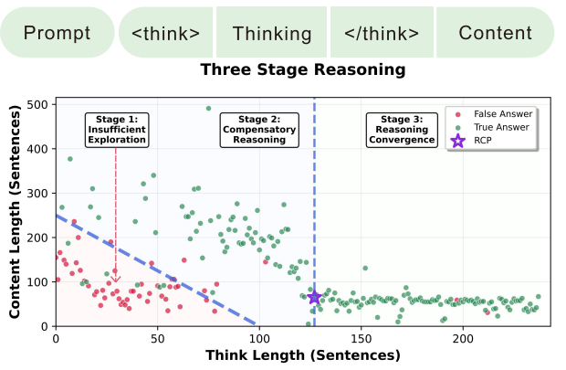
- Stop Spinning Wheels: Mitigating LLM Overthinking via Mining Patterns for Early Reasoning Exit (https://arxiv.org/pdf/2508.17627). The authors introduce a lightweight framework to detect and terminate reasoning at the optimal Reasoning Completion Point (RCP), preventing unnecessary token generation in large reasoning models. They categorize the reasoning process of LLMs into three stages: insufficient exploration, compensatory reasoning, and reasoning convergence. Typically, LLMs produce correct answers during the compensatory reasoning stage, while the reasoning convergence stage often triggers overthinking, leading to excessive resource usage or even infinite loops. The RCP is defined as the boundary marking the end of the compensatory reasoning stage and typically appears at the end of the first complete reasoning cycle, beyond which additional reasoning offers no accuracy gain. To balance efficiency and accuracy, the authors distilled insights from CatBoost feature importance analysis into a concise and effective set of stepwise heuristic rules. Experiments on benchmarks such as AIME24, AIME25, and GPQA-D demonstrate that the proposed strategy reduces token consumption by over 30% while maintaining or improving reasoning accuracy.
- A Systematic Analysis of Hybrid Linear Attention (https://arxiv.org/pdf/2507.06457). This work systematically analyzes hybrid linear attention architectures to balance computational efficiency with long-range recall in large language models. The authors construct hybrid models by interleaving linear and full attention layers at varying ratios (24:1, 12:1, 6:1, 3:1) to analyze their impact on performance and efficiency. The key insight is that gating, hierarchical recurrence, and controlled forgetting mechanisms are critical to achieve Transformer-level recall in hybrid architectures when deployed at a 3:1 to 6:1 linear-to-full attention ratio, reducing KV cache memory by a factor of 4-7x.
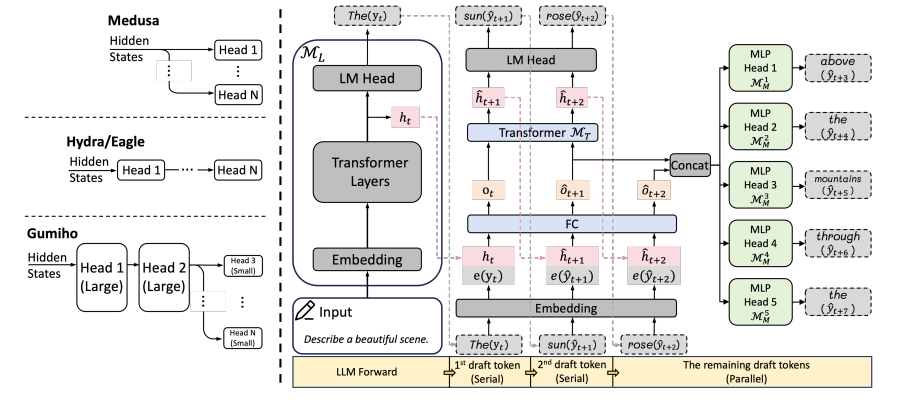
- Gumiho: A Hybrid Architecture to Prioritize Early Tokens in Speculative Decoding (https://arxiv.org/pdf/2503.10135). The authors deliver a new Speculative Decoding (SD) method for accelerating Large Language Model (LLM) inference. This is an incremental improvement of the Eagle SD method from NVIDIA. Its core insight is that early tokens in a speculative decoding draft are disproportionately more important than later ones. The paper introduces a novel hybrid architecture to exploit this: a high-accuracy serial Transformer for the crucial first tokens and efficient parallel MLPs for subsequent ones. Gumiho surpasses the existing SOTA method EAGLE-2 by 4.5%∼15.8%, but does not have a comparison with EAGLE-3. The code: https://github.com/AMD-AGI/Gumiho
Software
- OptiLLM (https://github.com/algorithmicsuperintelligence/optillm) is an OpenAI API-compatible optimizing inference proxy that implements 20+ state-of-the-art techniques to dramatically improve LLM accuracy and performance on reasoning tasks - without requiring any model training or fine-tuning. It is possible to beat the frontier models using these techniques across diverse tasks by doing additional compute at inference time.
- FlashDMoE (https://flash-moe.github.io): Fast Distributed MoE in a Single Kernel - a fully GPU-resident MoE operator that fuses expert computation and inter-GPU communication into a single persistent GPU kernel. FlashDMoE enables fine-grained pipelining of dispatch, compute, and combine phases, eliminating launch overheads and reducing idle gaps.
- LMCache (https://github.com/LMCache/LMCache) is an LLM serving extension that cuts TTFT and boosts throughput in long-context scenarios. By storing the KV caches of reusable texts across various locations, including (GPU, CPU DRAM, Local Disk), LMCache reuses the KV caches of any reused text (not necessarily prefix) in any serving engine instance. Integrated with vLLM, LMCache delivers 3–10× faster responses and lower GPU usage in tasks like multi-round QA and RAG.
- Flash Attention 4 (FA4) is a newly developed CUDA kernel optimized for Nvidia’s Blackwell architecture, delivering roughly a 20% performance improvement over previous versions. It achieves this speedup through an asynchronous pipeline of operations and several mathematical optimizations, including a fast exponential approximation and a more efficient online softmax. Tri Dao presented early results of FA4 at Hot Chips, and further implementation details were later shared in a blog post: https://modal.com/blog/reverse-engineer-flash-attention-4.
Q2'25: Technology Update – Low Precision and Model Optimization
Authors
Alexander Suslov, Alexander Kozlov, Nikolay Lyalyushkin, Nikita Savelyev, Souvikk Kundu, Andrey Anufriev, Pablo Munoz, Liubov Talamanova, Daniil Lyakhov, Yury Gorbachev, Nilesh Jain, Maxim Proshin, Evangelos Georganas
Summary
This quarter marked a major shift towards efficiency in large-scale AI, driven by the unsustainable computational and memory costs of current architectures. The focus is now on making models dramatically faster and more hardware-friendly, especially for demanding long-context and multimodal tasks. 🚀 There is a growing adoption of dynamic, data-aware techniques like dynamic sparse attention and token pruning, which intelligently reduce computation by focusing only on the most critical information. Furthermore, optimization is increasingly tailored to new hardware through ultra-low precision; quantization is being pushed to the extreme, with native 1-bit (BitNet) inference and 4-bit (FP4) training becoming viable by aligning directly with new GPU capabilities.
A parallel trend is the creation of simple, readable frameworks like Nano-vLLM, whose lightweight design aims to lower the barrier to entry for developers and researchers.
Highlights
- MMInference: Accelerating Pre-filling for Long-Context Visual Language Models via Modality-Aware Permutation Sparse Attention (https://arxiv.org/pdf/2502.02631). The authors introduce MMInference (Multimodality Million tokens Inference), a dynamic sparse attention method that accelerates the prefilling stage for long-context multi-modal inputs. The core ideas stemfrom analyzing the attention patterns specific to multi-modal inputs in VLMs: (1) Visual inputs exhibit strong temporal and spatial locality, leading to a unique sparse pattern the authors term the "Grid pattern".(2) Attention patterns differ significantly within a modality versus across modalities. The authors introduces the permutation-based method for offline searching the optimal sparse patterns for each head based on the input andoptimized kernels to compute attention much faster. MMInference speeds up the VLM pre-filling stage by up to 8.3x (at 1 million tokens) without losing accuracy and without needing any model retraining.The paper demonstrates maintained performance across various multi-modal benchmarks (like Video QA and Captioning) using state-of-the-art models (LongVila, LlavaVideo, VideoChat-Flash, Qwen2.5-VL). The code is available at https://aka.ms/MMInference.
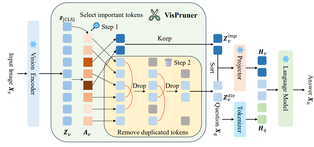
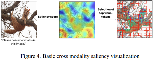
- Beyond Text-Visual Attention: Exploiting Visual Cues for Effective Token Pruning in VLMs (https://arxiv.org/pdf/2412.01818). The authors introduce VisPruner, a training-free method for compressing visual token sequences in VLMs, dramatically reducing computational overhead. Unlike prior approaches that rely on text-visual attention scores - often biased and dispersed - VisPruner leverages visual cues directly from the visual encoder. They identify two key flaws in attention-based pruning: (1) attention shift: positional bias causes attention to favor lower image regions (tokens closer to the text in sequence); (2) attention dispersion: attention is spread too uniformly, making it hard to identify important tokens. VisPruner first selects a small set of important tokens using [CLS] attention (typically focused on foreground objects), then complements them with diverse tokens selected via similarity-based filtering to preserve background and contextual information. This visual-centric pruning strategy avoids reliance on language model internals and is compatible with fast attention mechanisms like FlashAttention. VisPruner outperforms finetuning-free baselines like FastV, SparseVLM, and VisionZip across 13 benchmarks—including high-resolution and video tasks—even when retaining as little as 5% of the original visual tokens. It achieves up to 95% FLOPs reduction and 75% latency reduction.
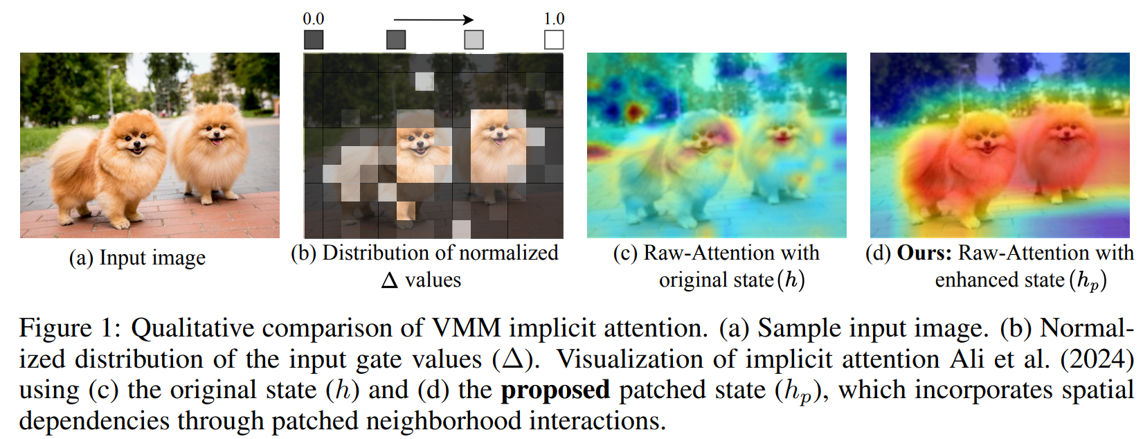
- OuroMamba: A Data-Free Quantization Framework for Vision Mamba Models (https://www.arxiv.org/pdf/2503.10959). The authors present OuroMamba, the first data-free post-training quantization (DFQ) method for vision Mamba-based models (VMMs). The authors identify two key challenges in enabling DFQ for VMMs, (1) VMM’s recurrent state transitions restricts capturing of long-range interactions and leads to semantically weak synthetic data,(2) VMM activation exhibit dynamic outlier variations across time-steps, rendering existing static PTQ techniques ineffective. To address these challenges, OuroMamba presents a two-stage framework: (1) OuroMamba-Gen to generate semantically rich and meaningful synthetic data. It applies constructive learning on patch level VMM features generated through neighborhood interactions in the latent state space, (2) OuroMamba-Quant to employ mixed-precision quantization with lightweight dynamic outlier detection during inference. In specific, the paper presents a threshold based outlier channel selection strategy for activation that gets updated every time-step. Extensive experiments across vision and generative tasks show that our data-free OuroMamba surpasses existing data-driven PTQ techniques, achieving state-of-the-art performance across diverse quantization settings. Additionally, the authors demonstrate the efficacy via implementation of efficient GPU kernels to achieve practical latency speedup of up to 2.36×.
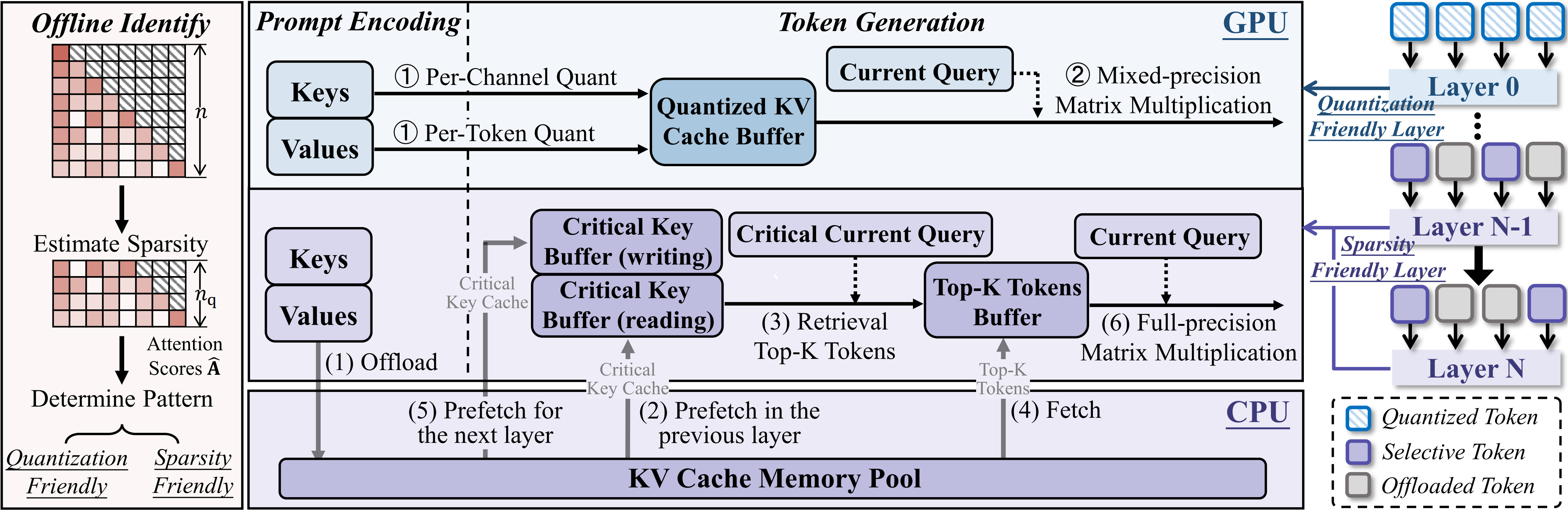
- TailorKV: A Hybrid Framework for Long-Context Inference via Tailored KV Cache Optimization (https://arxiv.org/pdf/2505.19586). TailorKV is a novel framework designed to optimize the KV cache in LLMs for long-context inference, significantly reducing GPU memory usage and latency without sacrificing model performance.Instead of applying a one-size-fits-all compression strategy, TailorKV intelligently tailors compression based on the characteristics of each Transformer layer. The authors look at how each layer distributes its attention across tokens: (1) If a layer spreads attention broadly across many tokens, it’s considered to be dense. These layers are good candidates for quantization, because compressing them doesn’t significantly harm performance (usually shallow layers). (2) If a layer focuses attention on just a few tokens, it’s considered to be sparse. These layers are better suited for sparse retrieval, where only the most important tokens are kept in memory (deeper layers). To make this decision, they compute a score for each layer that reflects how concentrated or spread out the attention is. If the score is above a certain threshold, the layer is labeled quantization-friendly; otherwise, it’s considered sparsity-friendly. This classification is done offline, meaning it’s calculated once before inference, so it doesn’t affect runtime performance. TailorKV drastically reduces memory usage by quantizing 1 to 2 layers to 1-bit precision and loading only 1% to 3% of the tokens for the remaining layers.Maintains high accuracy across diverse tasks and datasets, outperforming state-of-the-art methods like SnapKV, Quest, and PQCache on LongBench. Code is available at: https://github.com/ydyhello/TailorKV.
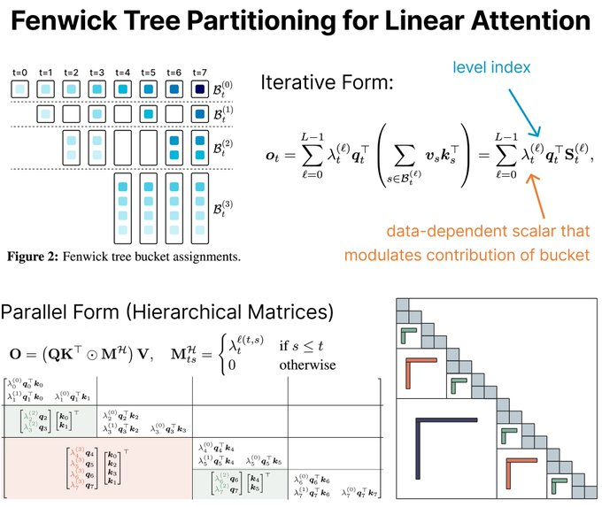
- Log-Linear Attention (https://arxiv.org/pdf/2506.04761). The authors present Log-Linear Attention, a general framework that extends linear attention and state-space models by introducing a logarithmic growing memory structure for efficient long-context modeling. The paper identifies two key limitations in prior linear attention architectures: (1) the use of fixed-size hidden states restricts their ability to model multi-scale temporal dependencies, and (2) their performance degrades on long sequences due to the lack of hierarchical context aggregation.To address these challenges, Log-Linear Attention places a particular structure on the attention mask, enabling the compute cost to be log-linear and the memory cost to be logarithmic in sequence length (O(TlogT) training time,O(logT) inference time and memory). Conceptually, it uses a Fenwick tree–based scheme to hierarchically partition the input into power-of-two-sized segments. Each query attends to a logarithmic number of hidden states, summarizing increasingly coarse ranges of past tokens. This design emphasizes recent context with finer granularity, while efficiently compressing distant information.The framework is instantiated on top of two representative models: Mamba-2 and Gated DeltaNet, resulting in Log-Linear Mamba-2 and Log-Linear Gated DeltaNet. These variants inherit the expressive recurrence structures of their linear counterparts but benefit from logarithmic memory growth and sub-quadratic training algorithms via a custom chunk-wise parallel scan implementation in Triton.Experiments across language modeling, long-context retrieval, and in-context reasoning benchmarks show that Log-Linear Attention consistently improves long-range recall while achieving competitive or better throughput than FlashAttention-2 at longer sequence lengths (>8K). The code is available at https://github.com/HanGuo97/log-linear-attention.
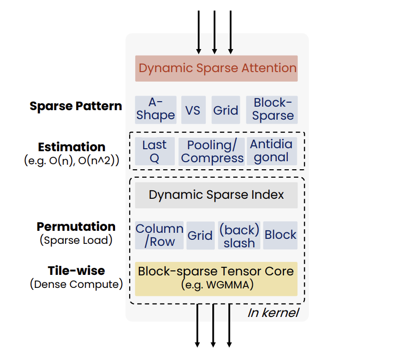
- The Sparse Frontier: Sparse Attention Trade-offs in Transformer LLMs (https://arxiv.org/pdf/2504.17768). The authors introduce SparseFrontier, a systematic evaluation of dynamic sparse attention methods aimed at accelerating inference in LLMs for long-context inputs (up to 128K tokens). The core ideas stem from an extensive analysis of sparse attention trade-offs across different inference stages, model scales, and task types: (1) Sparse attention during decoding tolerates higher sparsity than during prefilling, particularly in larger models, due to differences in memory and compute bottlenecks.(2) No single sparse pattern is optimal across all tasks - retrieval, aggregation, and reasoning tasks each require different units of sparsification (e.g., blocks vs. tokens) and budget strategies. During prefilling, the best sparsification structure (e.g., blocks or verticals and slashes) is task-dependent, with uniform allocation across layers performing comparably to dynamic allocation. During decoding, page-level Quest excels by preserving the KV cache structure, avoiding the performance degradation associated with token pruning during generation. Their FLOPS analysis shows that for long context, large sparse models outperform smaller dense ones at the same compute cost. They also establish scaling laws predicting accuracy from model size, sequence length, and compression ratio.The code is available at: https://github.com/PiotrNawrot/sparse-frontier.
Papers with notable results
Quantization
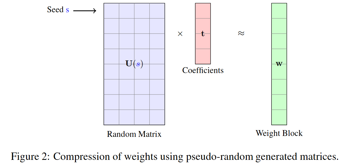
- SeedLM: Compressing LLM Weights into Seeds of Pseudo-Random Generators (https://arxiv.org/pdf/2410.10714). This paper introduces SeedLM, a novel data-free post-training compression method for Large Language Models (LLMs) that uses seeds of pseudo-random generators and some coefficients to recreate model weights. SeedLM aims to reduce memory access and leverage idle compute cycles during inference, effectively speeding up memory-bound tasks by trading compute for fewer memory accesses.The method generalizes well across diverse tasks, achieving better zero-shot accuracy retention at 4- and 3-bit compression compared to OmniQuant, AWQ and QuIP#. Additionally, FPGA-based tests demonstrate close to 4x speedup for memory-bound tasks such as generation for 4bit per value over an FP16 Llama baseline.
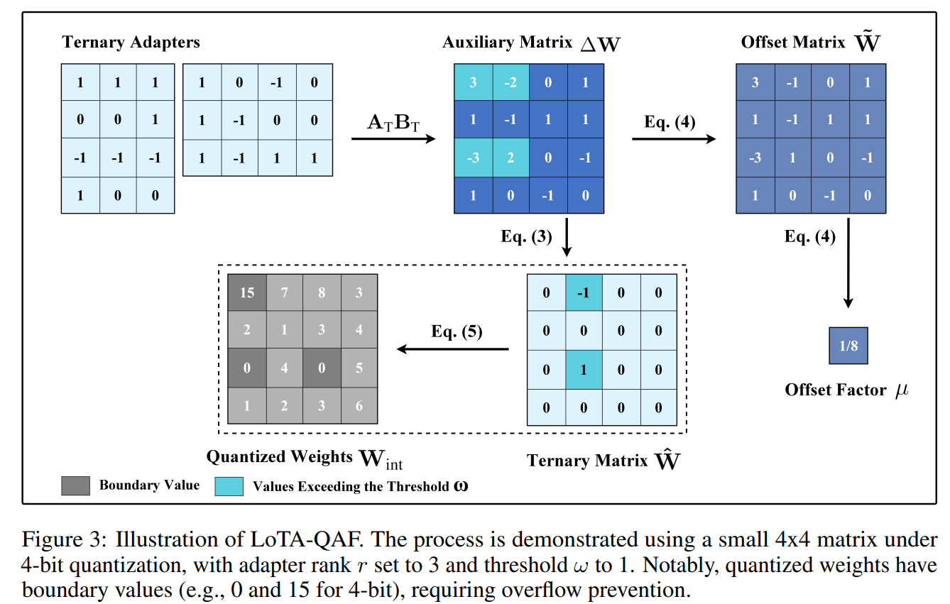
- LoTA-QAF: Lossless Ternary Adaptation for Quantization-Aware Fine-Tuning (https://arxiv.org/pdf/2505.18724). LoTA-QAF is a quantization-aware fine-tuning method for LLMs designed for efficient edge deployment. Its key innovation is a ternary adaptation approach, where ternary adapter matrices can only increment, decrement, or leave unchanged each quantized integer weight (+1, −1, or 0) within the quantization grid during fine-tuning. This tightly restricts the amount each quantized value can change, ensuring the adapters do not make large modifications to weights. The method enables lossless merging of adaptation into the quantized model, preserving computational efficiency and model performance with no quantization-induced accuracy loss at merge. The method uses a novel ternary signed gradient descent (t-SignSGD) optimizer to efficiently update these highly constrained ternary weights. Evaluated on the Llama-3.1/3.3 and Qwen-2.5 families, LoTA-QAF consistently outperforms previous quantization-aware fine-tuning methods such as QA-LoRA, especially at very low bit-widths (2-bit and 3-bit quantization), recovering up to 5.14% more accuracy on MMLU compared to LoRA under 2-bit quantization, while also being 1.7x–2x faster at inference after merging. Task-specific fine-tuning shows LoTA-QAF improves on other quantization-aware methods, though it slightly lags behind full-precision LoRA in those scenarios.The code is available at: https://github.com/KingdalfGoodman/LoTA-QAF.
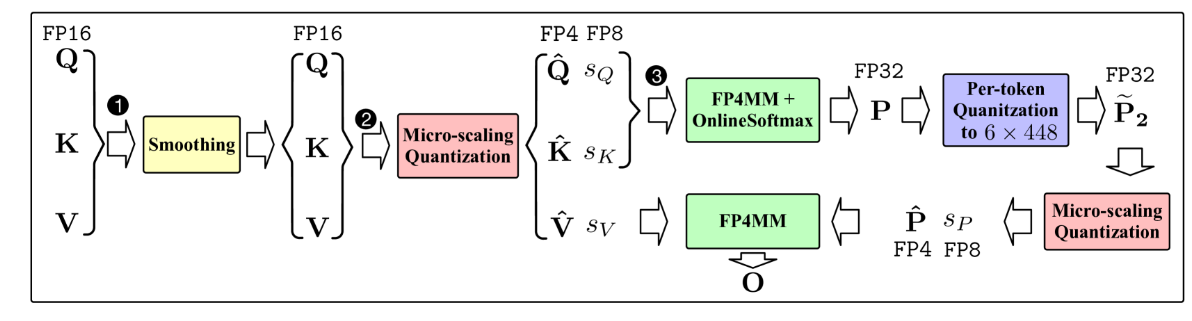
- SageAttention3: Microscaling FP4 Attention for Inference and An Exploration of 8-bit Training (https://arxiv.org/abs/2505.11594). The authors introduce SageAttention3, a novel FP4 micro-scaling quantization technique for Transformer attention designed to achieve a 5x speedup in inference on NVIDIA GPUs and an 8-bit novel training approach that preserves model accuracy during finetuning while reducing memory demands. The method applies FP4 quantization to the two main attention matrix multiplications, using a microscaling strategy with a group size of 16 elements per scale factor. This fine granularity limits the impact of outlier values that can otherwise cause significant quantization error. To address issues with quantizing the attention map, the authors propose a two-level quantization scheme. First, each row of attention map is scaled into the range[0, 448 × 6], which ensures the FP8 scaling factor (required by hardware) fully utilizes its representation range. Then, FP4 quantization is applied at the block level. This two-step process significantly reduces quantization error compared to direct quantization. Empirical results show that SageAttention3 delivers substantial inference speedups with minimal quality loss on language, image, and video generation benchmarks. The code is available at: https://github.com/thu-ml/SageAttention.
- MambaQuant: Quantizing the Mamba Family with Variance Aligned Rotation Methods (https://arxiv.org/abs/2501.13484). This paper tackles the challenge of post-training quantization for Mamba architectures. Standard quantization techniques adapted from large language models result in substantial accuracy loss when applied to Mamba models, largely due to extreme outliers and inconsistent variances across different channels in weights and activations. To address these issues, the authors propose MambaQuant, introducing two variance alignment techniques: KLT-Enhanced and Smooth-Fused rotations. These methods effectively equalize channel variances, resulting in more uniform data distributions before quantization. Experimental results show that MambaQuant enables Mamba models to be quantized to 8 bits for both weights and activations with less than 1% loss in accuracy, markedly surpassing previous approaches on both vision and language tasks.
- APHQ-ViT: Post-Training Quantization with Average Perturbation Hessian Based Reconstruction for Vision Transformers (https://arxiv.org/pdf/2504.02508). APHQ-ViT is a PTQ method designed to address the challenges of quantizing Vision Transformers, particularly under ultra-low bit settings. Traditional reconstruction-based PTQ methods, effective for Convolutional Neural Networks, often fail with ViTs due to inaccurate estimation of output importance and significant accuracy degradation when quantizing post-GELU activations. To overcome these issues, APHQ-ViT introduces an improved Average Perturbation Hessian (APH) loss for better importance estimation. Additionally, it proposes an MLP Reconstruction technique that replaces the GELU activation function with ReLU in the MLP modules and reconstructs them using the APH loss on a small unlabeled calibration set. Experiments demonstrate that APHQ-ViT, utilizing linear quantizers, outperforms existing PTQ methods by substantial margins in 3-bit and 4-bit quantization across various vision tasks. The source code for APHQ-ViT is available at https://github.com/GoatWu/APHQ-ViT.
- DL-QAT: Weight-Decomposed Low-Rank Quantization-Aware Training for Large Language Models (https://arxiv.org/abs/2504.09223). DL-QAT is a quantization-aware training (QAT) technique for LLMs that achieves high efficiency by updating less than 1% of parameters. It introduces group-specific quantization magnitudes and uses LoRA-based low-rank adaptation within the quantization space. Tested on LLaMA and LLaMA2, DL-QAT outperforms previous state-of-the-art methods—including QA-LoRA and LLM-QAT - by up to 4.2% on MMLU benchmarks for 3-bit models, while greatly reducing memory and training costs.
- BitNet b1.58 2B4T Technical Report (https://arxiv.org/abs/2504.09223). Microsoft Research released the weights for BitNet b1.58 2B4T, the first open-source, native 1-bit Large Language Model (LLM) at the 2-billion parameter scale and inference framework bitnet.cpp. The new 2B model demonstrates performance comparable to the Qwen 2.5 1.5B on benchmarks, while operating at 2x the speed and consuming 12x less energy.
- Quartet: Native FP4 Training Can Be Optimal for Large Language Models (https://arxiv.org/pdf/2505.14669). The authors introduced a new method "Quarter" for the stable 4-bit floating-point (FP4) training. There is specifically designed for the native FP4 hardware in NVIDIA's new Blackwell GPUs and achieved a nearly 2x speedup on the most intensive training computations compared to 8-bit techniques, all while maintaining "near-lossless" accuracy. The method outlines to perform a forward pass that minimizes MSE (based on QuEST) together with a backwardpass that is unbiased (based on Stochastic Rounding). The code of extremely efficient GPU-aware implementation https://github.com/IST-DASLab/Quartet
- InfiJanice: Joint Analysis and In-situ Correction Engine for Quantization-Induced Math Degradation in Large Language Models (https://arxiv.org/pdf/2505.11574). The authours investigates how quantization significantly harms the mathematical reasoning abilities of LLMs. The study reveals that quantization can degrade reasoning accuracy by up to 69.81% on complex benchmarks, with smaller models being more severely affected. Authors developed an automated pipeline to analyze and categorize the specific errors introduced by quantization. Based on these findings, they created a compact, targeted dataset named "Silver Bullet." The most notable result is that fine-tuning a quantized model on as few as 332 of these curated examples for just 3–5 minutes on a single GPU is sufficient to restore its mathematical reasoning accuracy to the level of the original, full-precision model.
Pruning/Sparsity
- Token Sequence Compression for Efficient Multimodal Computing (https://arxiv.org/pdf/2504.17892). The authors introduce a training-free method for compressing visual token sequences in visual language models (VLMs), significantly reducing computational costs. Instead of relying on attention-based “saliency”—a measure of how much attention a model gives to each token—they use simple clustering to group similar visual tokens and aggregate them. Their “Cluster & Aggregate” approach outperforms prior finetuning-free methods like VisionZip and SparseVLM across 8+ benchmarks, even when retaining as little as 11% of the original tokens. Surprisingly, random and spatial sampling also perform competitively, revealing high redundancy in visual encodings.
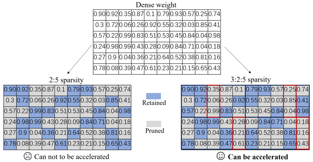
- Beyond 2:4: exploring V:N:M sparsity for efficient transformer inference on GPUs (https://arxiv.org/abs/2410.16135). This paper introduces and systematically studies V:N:M sparsity as a more efficient and flexible alternative to the industry-standard 2:4 sparsity for accelerating Transformer inference on GPUs. In the V:N:M approach, weight matrices are divided into V×M blocks; within each block, most columns are pruned, and 2:4 sparsity is then applied to the remaining columns. This scheme enables significantly higher and more adaptable sparsity ratios, while remaining compatible with existing GPU sparse tensor core acceleration. The authors propose a comprehensive framework for creating V:N:M-sparse Transformers: it features a heuristic method for selecting V and M values to optimize the accuracy-speedup trade-off, a V:N:M-specific channel permutation method for improving accuracy in low-budget training scenarios, and a three-stage LoRA training process for memory-efficient fine-tuning. Experimental results show that V:N:M-sparse Transformers can achieve much higher sparsity levels - such as 75% parameter reduction, while maintaining nearly lossless accuracy on downstream tasks, and outperform 2:4 sparsity in both speed and flexibility.
- TopV: Compatible Token Pruning with Inference Time Optimization for Fast and Low-Memory Multimodal Vision Language Model (https://arxiv.org/pdf/2503.18278v2). The authors introduce a training-free, optimization-based framework for reducing visual token redundancy in VLMs. Visual tokens often dominate the input sequence—up to 95% in some models. TopV addresses this by pruning unimportant visual tokens once during the prefilling stage, before decoding begins.Instead of relying on attention scores, TopV estimates the importance of each visual token by solving an optimal transport problem. In this setup: (1) Source tokens are the input visual tokens entering a specific transformer layer. (2) Target tokens are the output visual tokens after that layer has processed the input—specifically, the output after the Post-LN sub-layer. TopV calculates how much each input token contributes to the output using the Sinkhorn algorithm, guided by a cost function that considers: (1) How similar the tokens are in content (feature similarity), (2) How close they are in the image (spatial proximity), (3) How central they are in the image (centrality). To prevent visual collapse—especially in detail-sensitive tasks like OCR and captioning—TopV includes a lightweight recovery step. From the discarded tokens, TopV uniformly samples a subset at regular intervals (e.g., every 4th or 6th token) and reinserts them into the token sequence alongside the top-k tokens, ensuring spatial diversity and semantic coverage without significant overhead.TopV performs pruning once after the prompt and image are processed. The pruned visual token set remains fixed throughout decoding, enabling efficient and consistent inference.
- SparseVLM: Visual Token Sparsification for Efficient Vision-Language Model Inference (https://arxiv.org/pdf/2410.04417). SparseVLM introduces a lightweight, training-free framework for visual token sparsification in vision-language models (VLMs). Unlike text-agnostic approaches, it leverages cross-attention to identify text-relevant visual tokens (“raters”) and adaptively prunes others based on the rank of the attention matrix. Crucially, SparseVLM doesn’t discard all pruned tokens—instead, it recycles the most informative ones (those with high attention relevance scores). These are grouped using a density peak clustering algorithm, and each cluster is compressed into a single representative token. The reconstructed tokens are then reinserted into the model, replacing the larger set of pruned tokens with a compact, information-rich representation. Applied to LLaVA, SparseVLM achieves a 4.5× compression rate with only a 0.9% accuracy drop, reduces CUDA latency by 37%, and saves 67% memory. The code is available at https://github.com/Gumpest/SparseVLMs.
Other
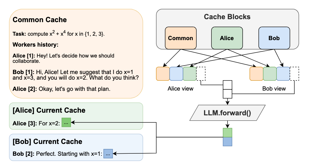
- Hogwild! Inference: Parallel LLM Generation via Concurrent Attention (https://arxiv.org/pdf/2504.06261). Hogwild! Inference introduces a novel paradigm for parallel inference for reasoning tasks that departs significantly from prior structured approaches by enabling dynamic, parallel collaboration. The method runs multiple LLM "workers" concurrently, allowing them to interact in real-time through a shared Key-Value (KV) cache. This shared workspace lets workers see each other's progress as it happens, fostering emergent teamwork without rigid, pre-planned coordination. A key innovation is the efficient use of Rotary Position Embeddings (RoPE) to synchronize the workers' views of the shared cache with minimal computational overhead. Empirical results show significant wall-clock speedups—up to 3.6x with 4 workers—on complex reasoning tasks. This is achieved "out of the box" on existing models without requiring fine-tuning and can be stacked with another optimization methods such as speculative decoding. The technique fundamentally improves the speed-cost-quality trade-off for inference, shifting the paradigm from sequential "chains of thought" to collaborative "teams of thought". The code is available at https://github.com/eqimp/hogwild_llm.
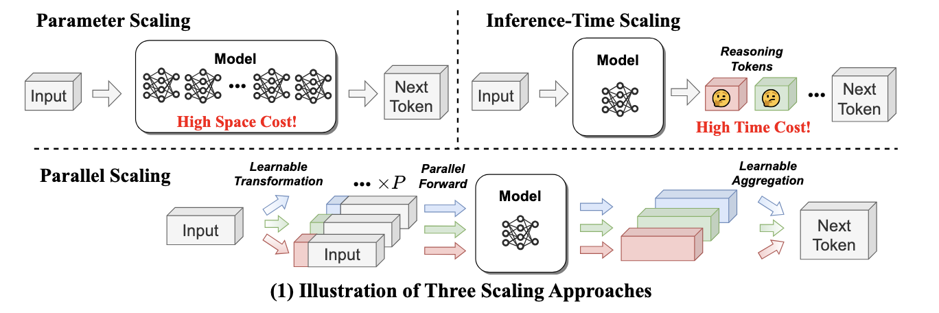
- Parallel Scaling Law for Language Models (https://arxiv.org/pdf/2505.10475). The authors introduce a novel "parallel" scaling method for LLMs (ParScale), distinct from traditional parameter (Dense, MoE) or inference-time (CoT) scaling. The technique processes a single input through 'P' parallel streams, each modified by a unique, learnable prefix vector. These streams are run concurrently on the same base model, and their outputs are intelligently aggregated by a small network. This method yields a quality improvement equivalent to increasing the model size by a factor of log(P), without actually expanding the core parameter count. For example, 8 parallel streams can match the performance of a model three times larger. ParScale is highly efficient for local inference, where memory bandwidth is the main bottleneck. Compared to direct parameter scaling for similar quality, it can require up to 22x less additional RAM and add 6x less latency. The approach can be applied for pretrained models, even with frozen weight, fine-tune only perscale components. The code is available at https://github.com/QwenLM/ParScale.
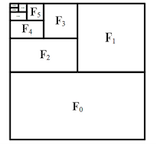
- Packing Input Frame Context in Next-Frame Prediction Models for Video Generation (https://arxiv.org/pdf/2504.12626). FramePack is a framework for next-frame prediction video generators that enables long-duration video synthesis with a constant computational cost (O(1)), regardless of length. It circumvents growing context windows by maintaining a fixed-size token buffer and codes input frames as shown in the figure below. To maintain temporal consistency and mitigate error accumulation, the system employs a bi-directional sampling scheme, alternating between forward and backward prediction passes. This efficiency allows a 13-billion parameter model to generate over 1800 frames (1 minute @ 30 fps) on a GPU with only 6GB of VRAM. The O(1) complexity in memory and latency makes FramePack a practical solution for generating minute-long videos on consumer hardware, with generation speeds of ~1.5 seconds per frame reported on an RTX 4090.The code is available at https://github.com/lllyasviel/FramePack.
- MoDM: Efficient Serving for Image Generation via Mixture-of-Diffusion Models (https://arxiv.org/pdf/2503.11972). Diffusion-based text-to-image generation models trade latency for quality: small models are fast but generate lower quality images, while large models produce better images but are slow. This paper presents MoDM, a novel caching-based serving system for diffusion models that dynamically balances latency and quality through a mixture of diffusion models.Unlike prior approaches that rely on model-specific internal features, MoDM caches final images, allowing seamless retrieval and reuse across multiple diffusion model families.This design enables adaptive serving by dynamically balancing latency and image quality: using smaller models for cache-hit requests to reduce latency while reserving larger models for cache-miss requests to maintain quality. Small model image quality is preserved using retrieved cached images. MoDM has a global monitor that optimally allocates GPU resources and balances inference workload, ensuring high throughput while meeting Service-Level Objectives (SLOs) under varying request rates. Extensive evaluations show that MoDM significantly reduces an average serving time by 2.5× while retaining image quality, making it a practical solution for scalable and resource-efficient model deployment.
- Fast-dLLM: Training-free Acceleration of Diffusion LLM by Enabling KV Cache and Parallel Decoding (https://arxiv.org/abs/2505.22618). Fast-dLLM is a training-free method to accelerate diffusion-based large language models by introducing a block-wise KV Cache and confidence-aware parallel decoding. The block-wise KV Cache reuses more than 90% of attention activations with bidirectional (prefix and suffix) caching, delivering throughput improvements ranging from 8.1x to 27.6x while keeping accuracy loss under 2%. Confidence-aware parallel decoding selectively generates tokens that exceed a set confidence threshold (like 0.9), achieving up to 13.3x speedup and preserving output coherence thanks to theoretical guarantees. Experimentally, Fast-dLLM achieves up to 27.6× end-to-end speedup on 1024-token sequences (e.g., LLaDA, 8-shot) and keeps accuracy within 2% of the baseline across major reasoning and code benchmarks including GSM8K, MATH, HumanEval, and MBPP.
- SANA-Sprint: One-Step Diffusion with Continuous-Time Consistency Distillation (https://arxiv.org/pdf/2503.09641). SANA-Sprint is a highly efficient text-to-image diffusion model designed for ultra-fast generation. Its core innovation is a hybrid distillation framework that combines continuous-time consistency models (sCM) with latent adversarial diffusion distillation (LADD). This approach drastically reduces inference requirements from over 20 steps to just 1-4. Key performance benchmarks establish a new state-of-the-art. In a single step, SANA-Sprint generates a 1024x1024 image with FID of 7.59. This is achieved with a latency of just 0.1 seconds on an NVIDIA H100 GPU and 0.31 seconds on a consumer RTX 4090. This makes it approximately 10 times faster than its competitor, FLUX-schnell, while also delivering higher image quality.The code is available at https://github.com/NVlabs/Sana.
Software
- FlashRNN: I/O-Aware Optimization of Traditional RNNs on modern hardware (https://arxiv.org/abs/2412.07752). FlashRNN extends traditional RNNs - such as LSTMs and GRUs - by introducing a parallelization scheme where the hidden state is divided into multiple smaller blocks, allowing for parallel computation similar to the head-wise processing in Transformers. The authors develop and open-source custom fused CUDA and Triton kernels that leverage the GPU memory hierarchy efficiently for both forward and backward passes, together with an automatic hardware-aware optimization framework. This approach achieves up to 50x speedup over vanilla PyTorch implementations, making RNNs competitive with Transformer-like models on modern GPUs. The code is available at: https://github.com/NX-AI/flashrnn.
- Nano-vLLM (https://github.com/GeeeekExplorer/nano-vllm). A lightweight vLLM implementation built from scratch.Key Features: (1)🚀 Fast offline inference - Comparable inference speeds to vLLM (2)📖 Readable codebase - Clean implementation in ~ 1,200 lines of Python code (3)⚡ Optimization Suite - Prefix caching, Tensor Parallelism, Torch compilation, CUDA graph, etc.
- NeMo-Inspector: A Visualization Tool for LLM Generation Analysis (https://arxiv.org/pdf/2505.00903). The authors introduce NeMo-Inspector, an open-source tool designed to simplify the analysis of synthetic datasets with integrated inference capabilities.
- FlashInfer: Efficient and Customizable Attention Engine for LLM Inference Serving (https://arxiv.org/pdf/2501.01005). The authors present FlashInfer: a customizable and efficient attention engine for LLM serving. FlashInfer tackles KV-cache storage heterogeneityusing block-sparse format and composable formats to optimize memory access and reduce redundancy, supports JIT compilation and load-balanced scheduling algorithm adjusts to dynamism of user requests while maintaining compatibility with CUDAGraph which requires static configuration. FlashInfer achieve29-69% inter-token-latency reduction compared to Triton, 28-30% latency reduction for long-context inference, and 13-17% speedup for LLM serving with parallel generation.The code is available at https://github.com/flashinfer-ai/flashinfer.
OpenVINO GenAI GGUF Feature Update
Authors: Su Yang, Tianmeng Chen, Hongbo Zhao
This blog focuses on OpenVINO GenAI GGUF Reader updates. The model link, usage and technical details are in the previous blog: OpenVINO GenAI Supports GGUF Model
-
1. New Model: Qwen3
Model Graph supports Qwen3 architecture: load attn_q_norm attn_k_norm weight and add rms_norm.
Validated models on CPU/GPU: Qwen3-0.6B-f16, Qwen3-0.6B-Q8_0, Qwen3-4B-Q4_K_M
2. New Pipeline Capabilities: OV Model Serialization and Logging Printing
The new enable_save_ov_model property enables serialization of the OV model generated from a GGUF model (including the tokenizer) to the same path as the GGUF file in XML/BIN format for reuse. After OV IR serialization, the path to the GGUF-converted OV model can be used directly as input.
Set environment variable to print loading and serializing time via OPENVINO_LOG_LEVEL. Example:
3. New Feature: GGUF Tokenizers and Detokenizers
Create a computation graph for tokenizers/detokenizers read from a GGUF file via the tokenizer node factory.
Validated models: SmolLM2-135M.F16.gguf, DeepSeek-R1-Distill-Qwen-1.5B-Q4_K_M.gguf, Llama-3.2-1B-Instruct-Q4_K_M.gguf, qwen2.5-0.5b-instruct-q4_0.gguf.
Downloading OV tokenizers IR and replacing the GGUF-converted OV tokenizer/detokenizer IR could be a workaround for generation anomalies.
4. Enhanced Support for GPU Plugin
Removes zero-point array modification workaround for Q4_0 weights. Supports dynamic quantization for GGUF-converted models.
Notes: Llama.cpp’s quantization GGUF block size differs from OpenVINO NNCF’s weight compression group size, so generation bias is expected. For better performance, using OV NNCF quantized model IR is recommended, as the GGUF reader still needs to dequantize Q4_0/Q4KM’s q6k tensor to FP16.
Sample Code Update:
Use GGUF file as the only input and save model via enable_save_ov_model.
Modify the file samples/cpp/text_generation/greedy_causal_lm.cpp of OV GenAI package (validated OV 25.3 nightly 20250727).
Running with GGUF:
For the first use, use the GGUF file as the only input; for subsequent uses, use the path to the GGUF-converted model as input.
Dynamic quantization support from GPU with XMX
Scope of this document
This article explains the behavior of dynamic quantization on GPUs with XMX, such as Lunar Lake, Arrow lake and discrete GPU family(Alchemist, Battlemage).
It does not cover CPUs or GPUs without XMX(such as Meteor Lake). While the dynamic quantization is supported on these platforms as well, the behavior may differ slightly.
What is dynamic quantization?
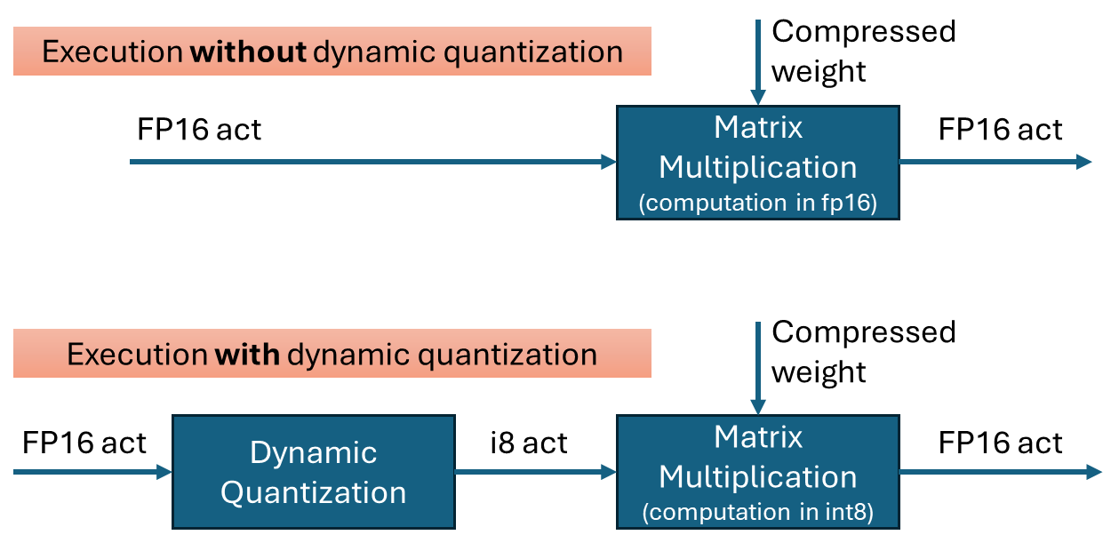
Dynamic quantization is a technique to improve the performance of transformer networks by quantizing the inputs to matrix multiplications. It is effective when weights are already quantized into int4 or int8. By performing the multiplication in int8 instead of fp16, computations can be executed faster with minimal loss in accuracy.
To perform quantization, the data is grouped, and the minimum and maximum values within each group are used to calculate the scale(and zero-point) for quantization. In OpenVINO’s dynamic quantization, this grouping occurs along the embedding axis (i.e., the innermost axis). The group size is configurable, as it impacts both performance and accuracy.
Default behavior on GPU with XMX for OpenVINO 2025.2
In the OpenVINO 2025.2 release, dynamic quantization is enabled by default for GPUs with XMX support. When a model contains a suitable matrix multiplication layer, OpenVINO automatically inserts a dynamic quantization layer before the MatMul operation. No additional configuration is required to activate dynamic quantization.
By default, dynamic quantization is applied per-token, meaning a unique scale value is generated for each token. This per-token granularity is chosen to maximize performance benefits.
However, dynamic quantization is applied conditionally based on input characteristics. Specifically, it is not applied when the token length is short—64 tokens or fewer.(That is, the row size of the matrix multiplication)
For example:
-If you run a large language model (LLM) with a short input prompt (≤ 64 tokens), dynamic quantization is disabled.
-If the prompt exceeds 64 tokens, dynamic quantization is enabled and may improve performance.
Note: Even in the long-input case, the second token is currently not dynamically quantized because row-size in matrix multiplication is small with KV cache.
Performance and Accuracy Impact
The impact of dynamic quantization on performance and accuracy can vary depending on the target model.
Performance
In general, dynamic quantization is expected to improve the performance of transformer models, including large language models (LLMs) with long input sequences—often by several tens of percent. However, the actual gain depends on several factors:
-Low MatMul Contribution: If the MatMul operation constitutes only a small portion of the model's total execution time, the performance benefit will be limited. For instance, in very long-context inputs, scaled-dot-product-attention may dominate the runtime, reducing the relative impact of MatMul optimization.
-Short Token Lengths: Performance gains diminish with shorter token lengths. While dynamic quantization improves compute efficiency, shorter inputs tend to be dominated by weight I/O overhead rather than compute cost.
Accuracy
Accuracy was evaluated using an internal test set and found to be within acceptable limits. However, depending on the model and workload, users may observe noticeable accuracy degradation.
If accuracy is a concern, you may:
-Disable dynamic quantization, or
-Use a smaller group size (e.g., 256), which can improve accuracy at some cost to performance.
How to Verify If dynamic quantization is Enabled on GPU with XMX
Since dynamic quantization occurs automatically under the hood, you may want to verify whether it is active. There are two main methods to check:
-Execution graph (exec-graph): The transformed graph generated by OpenVINO will include an additional "dynamic_quantize" layer if dynamic quantization is applied. You can inspect this by dumping the execution graph using the benchmark_app tool, assuming your model can be run with it. Please see the documentation for details: https://docs.openvino.ai/nightly/get-started/learn-openvino/openvino-samples/benchmark-tool.html
-Opencl-intercept-layer: You can view the list of executed kernels using the opencl-intercept-layer. Both call logging and device performance timing modes will show the "dynamic_quantize" kernel if it is executed. https://github.com/intel/opencl-intercept-layer
GraphTransformation with Dynamic Quantization
When dynamic quantization is enabled (i.e., dynamic_quantization_group_size != 0), a dynamic_quantize node is inserted before the target matrix multiplication nodes. (See the diagram above) Since the input length for LLMs is only known at inference time, the execution path is determined dynamically. If the input length is short (≤ 64 tokens), the dynamic_quantize node is skipped. For longer inputs, the node is executed to apply quantization.
If dynamic quantization is disabled (dynamic_quantization_group_size == 0), the dynamic_quantize node is not added to the graph at all.
Related properties
-dynamic_quantization_group_size: Sets the group size for dynamic quantization. In OpenVINO 2025.2, for GPUs with XMX, the default value is UINT64_MAX, which corresponds to per-token quantization.
For instructions on setting this property, please refer to: https://docs.openvino.ai/2025/openvino-workflow-generative/inference-with-optimum-intel.html#enabling-openvino-runtime-optimization
-OV_GPU_ASYM_DYNAMIC_QUANTIZATION: Enables asymmetric dynamic quantization. This means that in addition to the scale, a zero-point value is also computed during quantization. This setting is configured via an environment variable.
-OV_GPU_DYNAMIC_QUANTIZATION_THRESHOLD: Defines the minimum token length (or row size of the matrix) required to apply dynamic quantization. If the input token length is less than or equal to this value, dynamic quantization is not applied.
The default value is 64.
This setting can also be configured via an environment variable.
OpenVINO GenAI Supports GGUF Models
Authors: Fiona Zhao, Xiake Sun, Su Yang, Tianmeng Chen
1. Introduction:
This blog introduces the technical details of OpenVINO GenAI GGUF Reader and provides the Python and C++ implementations of OpenVINO GenAI pipeline that loads GGUF models, create OpenVINO graphs, and run GPU inference on-the-fly. To help customers integrate their existing llama.cpp-based LLM applications with OpenVINO inference, OpenVINO provides two approaches for GGUF support currently. Users can access the preview feature of the online GGUF Reader starting from the OpenVINO GenAI 2025.2 release.
GGUF (GGML Universal File Format) is the model format used by llama.cpp, a C/C++-based LLM inference framework. Models are typically trained in PyTorch, then converted and quantized into GGUF for use with llama.cpp.
The offline GGUF-to-OpenVINO approach converts and dequantizes the GGUF file into an FP16 PyTorch model. Subsequently, you can convert the PyTorch model into OpenVINO INT4 model via optimum-cli. The advantage of offline conversion is that it generates a unified OV model, which can be deployed with the C++/Python GenAI pipeline on different Intel platforms (including NPU). The drawback is the additional storage and processing overhead for PyTorch model dequantization and OV NNCF quantization. In this blog, we will focus on the second approach: Online GGUF Reader.
Key Features:
- - One-Step Loading: Directly read, unpack, and convert GGUF-compressed tensors to OpenVINO format in a single API call.
- - On-The-Fly Graph Creation: No intermediate PyTorch model and offline conversion with optimum-cli.
- - Integrated Dequantization: Handle dequantization during inference, eliminating extra storage and preprocessing steps.
- - Simplified Dependency Management: Zero PyTorch/Optimum dependencies.
2. Model library:
Validated model scope and platforms:
*Q8_0 GGUF is limited to MTL GPU, while FP16 GGUF works across MTL, LNL, and ARL GPUs.
Qwen/Qwen2.5-0.5B-Instruct-GGUF is a corner case, because Qwen2.5-0.5B-Q4KM contains a rarely used and unsupported q5_0 tensor.
In the OpenVINO GenAI 2025.2 release, the GGUF Reader does not support Qwen3 GGUF models. Support for Qwen3 GGUF is currently a work in progress (WIP) and will be added in a future update.
Our validation focuses on the widely used quantization type Q4_K_M.
Below is the list of Q4_K_M GGUF models validated on both CPU and GPU platforms (MTL, LNL, and ARL).
3. Usage:
OpenVINO GenAI provides implicit GGUF support based on the file extension, rather than through a separate GenAI GGUF sample. Users can create an LLMPipeline directly from a .gguf file.
Python Usage:
We provide a single Python script that downloads the GGUF model and runs it with the GenAI pipeline on-the-fly.
https://github.com/sammysun0711/openvino_aigc_samples/tree/gguf_ov_genai/GGUF-OV
C++ Usage:
Referring to this blog, How to Build OpenVINO™ GenAI APP in C++, build the OpenVINO GenAI pipeline using the OpenVINO Archive.
1. Download the latest OpenVINO Archive and Install dependencies.
Here, we use Windows to run qwen2.5-1.5b-instruct-q4_k_m.gguf as an example.
Once downloaded, unzip the downloaded file and extract the contents to <your_path>\openvino_genai_windows_2025.2.0.0.dev20250515_x86_64
2. Build OpenVINO GenAI example:
Open a command prompt and run setupvars.bat from the extracted OpenVINO GenAI folder.
<your_path>\openvino_genai_windows_2025.2.0.0.dev20250515_x86_64\setupvars.bat
Modify the file samples/cpp/text_generation/greedy_causal_lm.cpp to add GGUF file and OV tokenizer as input, and to enable GPU inference.
In the same command window, after the OpenVINO environment is initialized, navigate to the folder samples/cpp/, and run build_samples_msvc.bat.
Once the build process is complete, you will find the greedy_causal_lm.exe file in the path indicated in the build output.
3. Download LLM and Tokenizers
Download OpenVINO Tokenizers for Qwen2.5 models. (All Qwen2.5 parameter variants can share the same OpenVINO tokenizer IRs.)
Copy the above code into Notepad and save it as download_file.bat (ensure the file extension is .bat, not .txt). Run it by typing download_file.bat in the Command Prompt.
Or convert OpenVINO Tokenizers for the latest or other llama-based models (optional)
4. Run GGUF
4. Limitations
1.Tokenizer Conversion
In GenAI 2025.2, online conversion of GGUF tokenizers to OpenVINO (OV) format is not yet supported. This capability is a work in progress and is planned for inclusion in a future release.
As a workaround, we can download the OpenVINO tokenizer or perform offline conversion for use with the C++ pipeline, as shown in the usage section.
2.GPU INT8 kernel Group-size issues for q6_k and q8_0
Both Q4_0 model (last layer) and Q4KM GGUF model have q6_k GGUF tensor. Q8_0 GGUF has q8_0.
These GGUF-converted OpenVINO IR models work with CPU inference but fail on LNL and ARL GPUs.
OV INT8 is channel-wise by default, but q6_k’s group-size is 16, while q8_0’s group-size is 32. Currently INT8 dequantization has oneDNN issue.
To support Q4_0 and Q4KM, workaround for q6_k is to convert q6_k to f16 instead of q6_k-to-int8. This has an impact on Q4KM performance (most tensors of Q4KM are q4_k). It is recommended to use Q4_0 GGUF for better performance.
* Q8_0 has a oneDNN accuracy issue on LNL and ARL GPUs, and currently, no workaround is available for these platforms.
5. Technical Details
OpenVINO GenAI GGUF Reader: Simplify LLM deployment with direct GGUF model loading and optimized inference. No PyTorch dependencies, no additional conversions with intermediate PyTorch model, just high-performance inference out of the box.
Future Architecture Workflow:
In GenAI 25.2, the LLMPipeline reads GGUF files during each initialization by default. In addition to supporting online tokenizer conversion, future updates will introduce optimizations to the GGUF LLMPipeline with configuration option to save converted OpenVINO models.
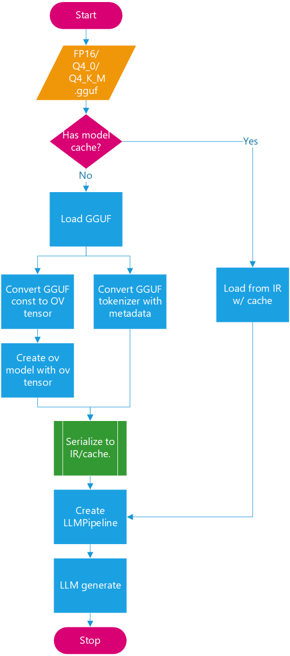
With the architecture defined, attention turns to the quantization formats.
To analyze the characteristics of Q4_K_M, it is helpful first to distinguish it from Q4_0, Q4_1, and Q8_0. These are lightweight, pure 4- or 8-bit quantization formats designed primarily for fast loading and minimal model size.
In contrast, Q4_K_M adopts a mixed-precision 4/6-bit scheme with a super-block structure that incorporates both block_scale and block_min, enabling higher accuracy while maintaining a compact footprint.
A deeper understanding of Q4_K_M can be achieved by comparing it directly with Q4_0. Notably, Q4_K_M encompasses two distinct GGUF tensor types: q4_k and q6_k. These tensors differ not only in precision but also in group size.
* Both Qwen2.5 Q4_0 and Q4KM GGUF have q6_k GGUF tensor. Q4_0 model’s last layer “output.weight” is the only one q6_k tensor.
-
So, what does this look like in practice? Qwen2.5 offers a clear example.
Qwen2.5 Q4_0 and Q4_K_M GGUF models both include q6_k tensors. In Q4_0, the only q6_k tensor is typically the final layer (output.weight). While OpenVINO shares embedding weights with lm_head, GGUF keeps them separate. For certain Qwen Q4_0 models (e.g., 3B/7B), lm_head is stored as a q6_k tensor in GGUF. To align with llama.cpp behavior and improve accuracy, this weight is loaded directly from GGUF instead of using shared embeddings.
Since INT6 is not supported by OpenVINO, all q6_k tensors are converted to INT8 for both Q4_0 and Q4_K_M models. Currently, to bypass GPU limitations with group-wise INT8 dequantization, q6_k tensors are converted to FP16 at load time on CPU. The q6_k workaround introduces some loading and inference performance overhead.
Q4_K_M models typically contain approximately six times more q4_k tensors than q6_k tensors. As a result, q6_k to fp16 workaround is relatively acceptable in terms of performance impact.
By leveraging common optimization techniques during the model loading phase, the overall pipeline latency can be further minimized.
Loading optimizations:
- - Parallel Parsing: Uses ov::parallel_for for multi-threaded.
- - Split-File Support: Compatible with llama.cpp’s sharding scheme for loading large GGUF models.
Loading performance results show that the Qwen2.5-7B-Q4_K_M model can be extracted and generated into an OpenVINO model graph in under 10 seconds on an Intel LNL U7 268V, dramatically outperforming the offline GGUF-to-OpenVINO approach, which takes about 4 minutes and over 15 GB of memory to save the PyTorch FP16 model (e.g., Llama-3.1-8b-Q4_K_M).
Thank you to all authors! Additionally, thanks to Kozlov, Alexander, and Lavrenov, Ilya for their contributions to the GGUF reader.
Dynamic shapes support in OpenVINO JIT compiler boosts inference performance by 40%
Authors: Ivan Novoselov, Alexandra Sidorova, Vladislav Golubev, Dmitry Gorokhov
Introduction
Deep learning (DL) has become a powerful tool for addressing challenges in various domains like computer vision, generative AI, and natural language processing. Industrial applications of deep learning often require performing inference in resource-constrained environments or in real time. That’s why it’s essential to optimize inference of DL models for particular use cases, such as low-latency, high-throughput or low-memory environments. Thankfully, there are several frameworks designed to make this easier, and OpenVINO stands out as a powerful tool for achieving these goals.
OpenVINO is an open-source toolkit for optimization and deployment of DL models. It demonstrates top-tier performance across a variety of hardware including CPU (x64, ARM), AI accelerators (Intel NPU) and Intel GPUs. OpenVINO supports models from popular AI frameworks and delivers out-of-the box performance improvements for diverse applications (you are welcome to explore demo notebooks). With ongoing development and a rapidly growing community, OpenVINO continues to evolve as a versatile solution for high-performance AI deployments.
The primary objective of OpenVINO is to maximize performance for a given DL model. To do that, OpenVINO applies a set of hardware-dependent optimizations The optimizations are typically performed by replacing a target group of operations with a custom operation that can be executed more efficiently. In the standard approach, these custom operations are executed using handcrafted implementations. This approach is highly effective when optimizing a few patterns of operations. On the other hand, it lacks scalability and thus requires too much effort when dozens of similar patterns should be supported.
To address this limitation and build a more flexible optimization engine, OpenVINO introduced Snippets, an integrated Just-In-Time (JIT) compiler for computational graphs. Snippets provide a flexible and scalable approach for operation fusions and enablement. The graph compiler automatically identifies subgraphs of operations that can benefit from fusion and combines them into a single node, referred to as “Subgraph”. Snippets then apply a series of optimizing transformations to the subgraph and JIT compile an executable that efficiently performs the computations defined by the subgraph.
One of the most common examples of such subgraphs is Scaled Dot-Product Attention (SDPA) pattern. SDPA it is a cornerstone of transformer-based architectures which dominate most of the state-of-the-art models. There are numerous SDPA pattern flavours and variations dictated by model-specific adjustments or optimizations. Thanks to compiler-based design, Snippets support most of these configurations. Fig. 1 illustrates the general structure of the SDPA pattern supported by Snippets, highlighting its adaptability to different model requirements:
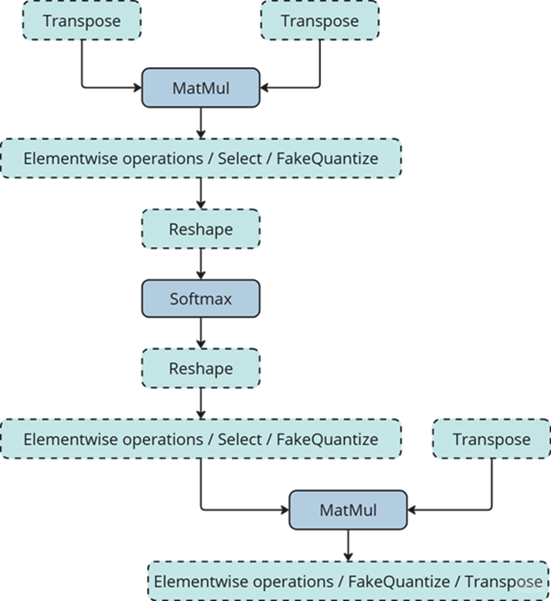
Note that SDPA has quadratic time and memory complexity with respect to sequence length. It means that by fusing SDPA-like patterns, Snippets significantly reduce memory consumption and accelerate transformer models, especially for large sequence lengths.
Snippets effectively optimized SDPA patterns but had a key limitation: they did not support dynamic shapes. In other words, input shapes must be known at the model compilation stage and can’t be changed in runtime. This limitation reduced the applicability of Snippets to many real-world scenarios where input shapes are not known in advance. While it is technically possible to JIT-compile a new binary for each unique set of input shapes, this approach introduces significant recompilation overheads, often negating the performance gains from SDPA fusion.
Fortunately, this static-shape limitation is not inherent to Snippets design. They can be modified to support dynamic shapes internally and generate shape-agnostic binaries. In this post, we discuss Snippets architecture and the challenges we faced during this dynamism enablement.
Architecture
The first step of the Snippets pipeline is called Tokenization. It is applied to an ov::Model, which represents OpenVINO Intermediate Representation (IR). It’s a standard IR in the OV Runtime you can read more about it here or here. The purpose of this stage is to identify parts of the initial model that can be lowered by Snippets efficiently. We are not going to discuss Tokenization in detail because this article is mostly focused on the dynamism implementation. A more in-depth description of the Tokenization process can be found in the Snippets design guide. The key takeaway for us here is that the subsequent lowering is performed on a part of the initial ov::Model. We will call this part Subgraph, and the Subgraph at first is also represented as an ov::Model.
Now let’s have a look at the lowering pipeline, its schematic representation is shown on Fig.2a. As can be seen from the picture, the lowering process consists of three main phases: Data Flow Optimizations, Control Flow Optimizations and Binary Code Generation. Let’s briefly discuss each of them.
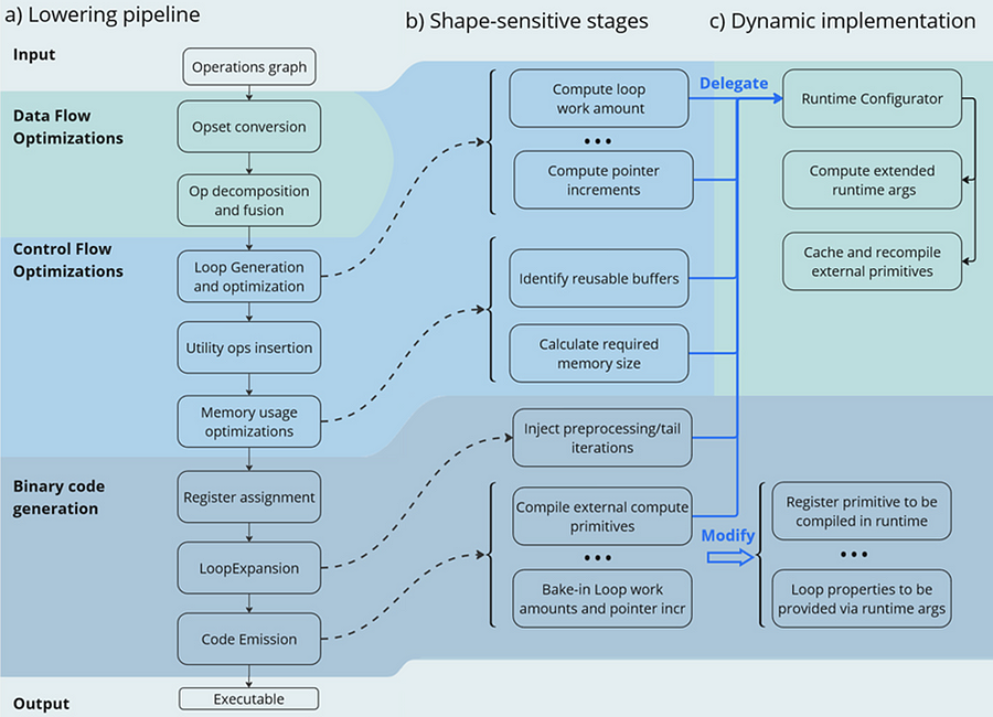
Lowering Pipeline
The first stage is the Data Flow optimizations. As we mentioned above, this stage’s input is a part of the initial model represented as an ov::Model. This representation is very convenient for high-level transformations such as opset conversion, operations’ fusion/decomposition and precision propagation. Here are some examples of the transformations performed on this stage:
- ConvertPowerToPowerStatic — operation Power with scalar exponent input is converted to PowerStatic operation from the Snippets opset. The PowerStatic ops then use the values of the exponents to produce more optimal code.
- FuseTransposeBrgemm — Transpose operations that can be executed in-place with Brgemm blocks are fused into the Brgemm operations.
- PrecisionPropagation pass automatically inserts Converts operations between the operations that don’t natively support the desired execution precision.
The next stage of the lowering process is Control Flow optimizations (or simply CFOs). Note that the ov::Model is designed to primarily describe data flow, so is not very convenient for CFOs. Therefore, we had to develop our own IR (called Linear IR or simply LIR) that explicitly represents both control and data flows, you can read more about LIR here. So the ov::Model IR is converted to LIR before the start of the CFOs.
As you can see from the Fig.2a, the Control Flow optimization pipeline could roughly be divided into three main blocks. The first one is called Loop Generation and Optimization. This block includes all loop-related optimizations such as automatic generation of loops based on the input tensors’ dimensions, loop fusion and blocking loops generation.
The second block of Control Flow optimizations is called Utility Ops Insertion. We need this block of transformations here to insert utility operations that depend on loop control structures, specifically on their entry and exit points locations. For example, operations like Load, Store, MemoryBuffer, LoopBegin and LoopEnd are inserted during this stage.
The last step of CFO is the Memory Usage Optimizations block. These transformations determine required sizes of internal memory buffers, and analyze how much of that memory can be reused. A graph coloring algorithm is employed to minimize memory consumption.
Now all Control Flow optimizations are performed, and we are ready to proceed to the next stage of the lowering pipeline — Binary Code Generation (BCG). As one can see from Fig.2a, this stage consists of three substages. The first one is Register Assignment. We use a fairly standard approach here: calculate live intervals first and use the linear scan algorithm to assign abstract registers that are later mapped to physical ones.
The next BSG substage is Loop Expansion. To better understand its purpose, let’s switch gears for a second and think about loops in general. Sometimes it’s necessary to process the first or the last iteration of a loop in a special way. For example, to initialize a variable or to process blocking loops’ tails. The Loop Expansion pass unrolls these special iterations (usually the first or the last one) and explicitly injects them into the IR. This is needed to facilitate subsequent code emission.
The final step of the BCG stage is Code Emission. At this stage, every operation in our IR is mapped to a binary code emitter, which is then used to produce a piece of executable code. As a result, we produce an executable that performs calculations described by the initial input ov::Model.
Dynamic Shapes Support
Note that some stages of the lowering pipeline are inherently shape-sensitive, i.e. they rely on specific values of input shapes to perform optimizations. These stages are schematically depicted on the Fig. 2b.
As can be seen from the picture, shapes are used to determine loops’ work amounts and pointer increments that should be performed on every iteration. These parameters are later baked into the executable during Code Emission. Another example is Memory Usage Optimizations, since input shapes are needed to calculate memory consumption. Loop Expansion also relies on input shapes, since it needs to understand if tail processing is required for a particular loop. Note also that Snippets use compute primitives from third-party libraries, BRGEMM block from OneDNN for example. These primitives should as well be compiled with appropriate parameters that are also shape-sensitive.
One way to address these challenges is to rerun the lowering pipeline for every new set of input shapes, and to employ caching to avoid processing the same shapes twice. However, preliminary analysis indicated that this approach is too slow. Since this re-lowering needs to be performed in runtime, the performance benefit provided by Snippets is essentially eliminated by the recompilation overheads.
The performed experiments thus indicate that we can afford to run the whole lowering pipeline only once during the model compilation stage. Only some minor adjustments can be made at runtime. In other words, we need to remove all shape-sensitive logic from the lowering pipeline and perform the compilation without it. The remaining shape-sensitive transformations should be performed at runtime. Of course, we would also need to share this runtime context with the compiled shape-agnostic kernel. The idea behind this approach is schematically represented on Fig. 2c.
As one can see from the picture, all the shape-sensitive transformations are now performed by a new entity called Runtime Configurator. It’s probably easier to understand its purpose in some examples.
Imagine that we need to perform a unary operation get_result(X) on an input tensor X — for example, apply an activation function. To do this, we need to load some input data from memory into registers, perform the necessary computations and write the results back to memory. Of course this read-compute-write sequence should be done in a loop since we need to process the entire input tensor. These steps are described in more detail in Fig. 3 using pseudocode. Fig. 3a corresponds to a static kernel while Fig. 3b represents a dynamic one.
Let’s consider the static kernel as a starting point. As the first step, we need to load pointers to input and output memory blobs to general-purpose registers (or simply GPRs) denoted G_IN and G_OUT on the picture. Then we initialize another GPR that stores the loop work amount (G_WA). Note that the loop is used to traverse the input tensor, so the loop’s work amount is fixed because the tensor’s dimensions are also known at the BCG stage. The next six steps in the picture (3 to 8) are in the loop’s body.
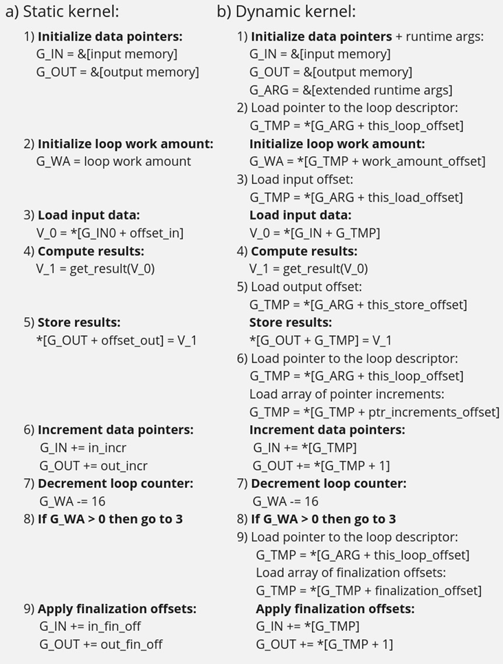
In step 3, we load input data into a vector register V_0, note that the appropriate pointer is already loaded to G_IN, and offset_in is fixed because the input tensor is static. Next, we apply our get_result function to the data in V_0 and place the result in a spare vector register V_1. Now we need to store V_1 back to memory, which is done on step 5. Note that offset_out is also known in the static case. This brings us almost to the end of the loop’s body, and the last few things we need to do are to increment data pointers (step 6), decrement loop counter (step 7), and jump to the beginning of the body, if needed (step 8).
Finally, we need to reset data pointers to their initial values after the loop is finished, which is done using finalization offsets on step 9. Note that this step could be omitted in our simplified example, but it’s often needed for more complicated use cases, such as when the data pointers are used by subsequent loops.
Now that we understand the static kernel, let’s consider the dynamic one, which is shown in Fig. 3b. Unsurprisingly, the dynamic kernel performs essentially the same steps as the static one, but with additional overhead due to loading shape-dependent parameters from the extended runtime arguments. Take step 1 as an example, we need to load not only memory pointers (to G_IN and G_OUT), but also a pointer to the runtime arguments prepared by the runtime configurator (to G_ARG).
Next, we need to load a pointer to the appropriate loop descriptor (a structure that stores loops’ parameters) to a temporary register G_TMP, and only then we can initialize the loop’s work amount register G_WA (step 2). Similarly, in order to load data to V_0, we need to load a runtime-calculated offset from the runtime arguments in step 3. The computations in step 4 are the same as in the static case, since they don’t depend on the input shapes. Storing the results to memory (step 5) requires reading a dynamic offset from the runtime arguments again. Next, we need to shift the data pointers, and again we have to load the increments from the corresponding loop descriptor in G_ARG because they are also shape-dependent, as the input tensor can be strided. The following two steps 7 and 8 are the same as in the static case, but the finalization offsets are also dynamic, so we have to load them from G_ARG yet again.
As one can see from Fig. 3, dynamic kernels incorporate additional overhead due to reading the extended runtime parameters provided by the runtime configurator. However, this overhead could be acceptable as long as the input tensor is large enough (Load/Store operations would take much longer than reading runtime arguments from L1) and the amount of computation is sufficient (get_results is much larger than the overhead). Let’s consider the performance of this design in the Results section to see if these conditions are met in practical use cases.
Results
We selected three platforms to evaluate the dynamic pipeline’s performance in Snippets. These platforms represent different market segments: the Intel Core machine is designed for high-performance user and professional tasks. While the Intel Xeon is a good example of enterprise-level hardware often used in data centers and cloud computing applications. The information about the platforms is described in the table below:
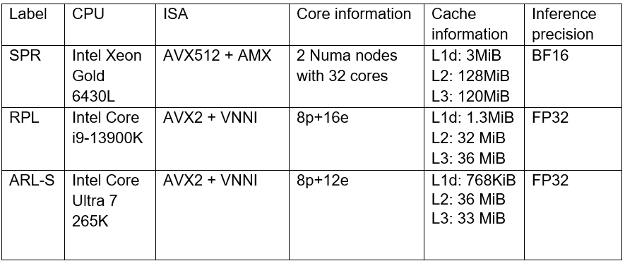
As discussed in the Introduction, Snippets support various SDPA-like patterns which form the backbone of Transformer models. These models often work with input data of arbitrary size (for example, sequence length in NLP). Thus, dynamic shapes support in Snippets can efficiently accelerate many models based on Transformer architecture with dynamic inputs.
We selected 43 different Transformer-models from HuggingFace to measure how the enablement of dynamic pipeline in Snippets affects performance. The models were downloaded and converted to OpenVINO IRs using Optimum Intel. These models represent different domains and were designed to solve various tasks in natural language processing, text-to-image image generation and speech recognition (see full model list at the end of the article). What unifies all these models is that they all contain SDPA subgraph and thus can be accelerated by Snippets.
Let’s take a closer look at the selected models. The 37 models of them solve different tasks in natural language processing. Their performance was evaluated using a list of 2000 text sequences with different lengths, which also mimics the real-word scenario. The total processing time of all the sequences were measured in every experiment. Note that the text sequences were converted to model inputs using model-specific tokenizers prior to the benchmarking. The lengths’ distribution of the tokenized sequences is shown on Fig. 4. As can be seen from the picture, the distribution is close to normal with the mean length of 31 tokens.
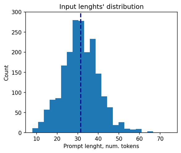
The other 6 models of the selected model scope solve tasks in text-to-image image generation (Stable Diffusion) and speech recognition (Whisper). These models decompose into several smaller models after export to OpenVINO representation using Optimum Intel. Stable Diffusion topology is decomposed into Encoder, Diffuser and Decoder. The most interesting model here is Diffuser because it’s the one responsible for denoising of the latent image representation. This generation stage is repeated several times, so it is the most computationally intensive, which mostly effects on the generation time of the image. Whisper is also decomposed into Encoder and Decoder, which also contain SDPA patterns. The Encoder encodes the spectrogram from the feature extractor to form a sequence of encoder hidden states. Then, the decoder autoregressively predicts text tokens, conditional on both the previous tokens and the encoder hidden states. Currently, Snippets support efficient execution of SDPA only in Whisper Encoder, while Decoder is a subject for future support. To evaluate the inference performance of Stable Diffusion and Whisper models, we collect generation time of image/speech using LLM Benchmark from openvino.genai. This script provides a unified approach to estimate performance for GenAI workloads in OpenVINO.
Performance Improvements
Note that the main goal of these experiments is to estimate the impact of Snippets on the performance of the dynamic pipeline. To do that, we performed two series of experiments for every model. The first version of experiments is with disabled Snippets tokenization. In this case, all operations from the SDPA pattern are performed on the CPU plugin side as stand-alone operations. The second variant of experiments — with enabled Snippets tokenization. The relative difference between numbers collected on these two series of experiments is our performance metric — speedup, the higher the better. Firstly, let’s take a closer look at the resulting speedups for the BERT models which are depicted on Fig. 5.
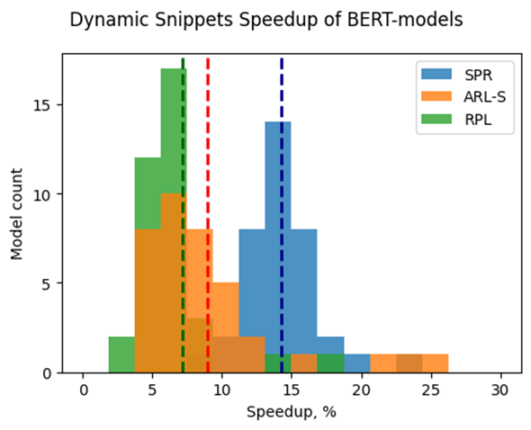
The speedups on RPL range from 3 to 18%, while on average the models are accelerated by 7%. The ARL-S speedups are somewhat higher and reach 20–25% for some models, the average acceleration factor is around 9%. The most affected platform is SPR, it has the highest average speedup of 15 %.
One can easily see from these numbers that both average and maximum speedups depend on the platform. To understand the reason for this variation, we should recall that the main optimizations delivered by Snippets are vertical fusion and tiling. These optimizations improve cache locality and reduce the memory access overheads. Note SPR has the largest caches among the examined platforms. It also uses BF16 precision that takes two times less space per data element compared to F32 used on ARL-S and RPL. Finally, SPR has AMX ISA extension that allows it to perform matrix multiplications much faster. As a result, SDPA execution was more memory bound on SPR, so this platform benefited the most from the Snippets enablement. At the same time, the model speedups on ARL-S and RPL are almost on the same level. These platforms use FP32 inference precision while SPR uses BF16, and they have less cache size than SPR.
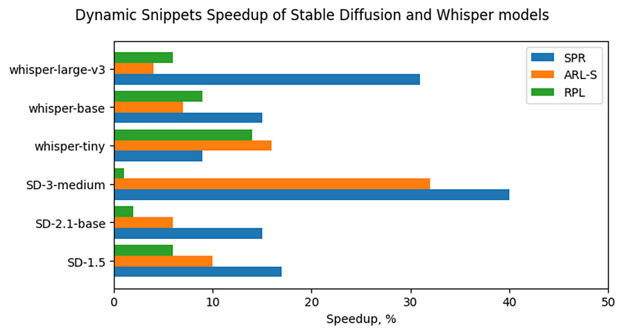
Now, let’s consider Stable Diffusion and Whisper topologies and compare their speedups with some of BERT-like models. As can be seen from the Fig. 6, the most accelerated Stable Diffusion topology is StableDiffusion-3-medium — almost 33% on ARL-S and 40% on SPR. The most accelerated model in this Stable Diffusion pipeline is Diffuser. This model has made a great contribution to speeding up the entire image generation time. The reason the Diffuser benefits more from Snippets enablement is that they use larger sequence lengths and embedding sizes. It means that their attention blocks process more data and are more memory constrained compared to BERT-like models. As a result, the Diffuser models in Stable Diffusion benefit more from the increased cache locality provided by Snippets. This effect is more pronounced on the SPR than on the ARL-S and RPL for the reasons discussed above (cache sizes, BF16, AMX).
The second most accelerated model is whisper-large-v3–30% on SPR. This model has more parameters than base and tiny models and process more Mel spectrogram frequency bins than they. It means that Encoder of whisper-large-v3 attention blocks processes more data, like Diffuser part of Stable Diffusion topologies. By the same reasons, whisper-large-v3 benefits more (increased cache locality provided by Snippets).
Memory Consumption Improvements
Another important improvement from Snippets using is reduction of memory consumption. Snippets use vertical fusion and various optimizations from Memory Usage Optimizations block (see the paragraph “Lowering Pipeline” in “Architecture” above for more details). Due to this fact, Subgraphs tokenized by Snippets consumes less memory than the same operations performed as stand-alone in CPU Plugin.
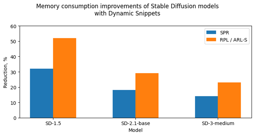
Let’s take a look at the Fig. 7 where we can see improvements in image generation memory consumption using Stable Diffusion pipelines from Snippets usage. As discussed above, the attention blocks in the Diffuser models from these pipelines process more data and consume more memory. Because of that, the greatest impact on memory consumption from using Snippets is seen on Stable Diffusion pipelines. For example, memory consumption of image generation is reduced by 25–50% on RPL and ARL-S platforms with FP32 inference precision and by 15–30% on SPR with BF16 inference precision.
Thus, one of the major improvements from using Snippets is memory consumption reduction. It allows extending the range of platforms which are capable to infer such memory-intensive models as Stable Diffusion.
Conclusion
Snippets is a JIT compiler used by OpenVINO to optimize performance-critical subgraphs. We briefly discussed Snippets’ lowering pipeline and the modifications made to enable dynamism support. After these changes, Snippets generate shape-agnostic kernels that can be used for various input shapes without recompilation.
This design was tested on realistic use cases across several platforms. As a result, we demonstrate that Snippets can accelerate BERT-like models by up to 25%, Stable Diffusion and Whisper pipelines up to 40%. Additionally, Snippets can significantly reduce memory consumption by several tens of percent. Notably, these improvements result from more optimal hardware utilization, so the models’ accuracy remains unaffected.
References
Model list can be found here: https://gist.github.com/a-sidorova/2c2aa584922389138e5ccbad0e0c773b
Intel Xeon Gold 6430L: https://www.intel.com/content/www/us/en/products/sku/231737/intel-xeon-gold-6430-processor-60m-cache-2-10-ghz/specifications.html
Intel Core i9-13900K: https://www.intel.com/content/www/us/en/products/sku/230496/intel-core-i913900k-processor-36m-cache-up-to-5-80-ghz/specifications.html
Intel Core Ultra 7 265K: https://www.intel.com/content/www/us/en/products/sku/241063/intel-core-ultra-7-processor-265k-30m-cache-up-to-5-50-ghz/specifications.html
Notices & Disclaimers
Performance varies by use, configuration, and other factors. Learn more on the Performance Index site.
No product or component can be absolutely secure. Your costs and results may vary. Intel technologies may require enabled hardware, software or service activation.
© Intel Corporation. Intel, the Intel logo, and other Intel marks are trademarks of Intel Corporation or its subsidiaries.
OpenVINO.GenAI Delivers C API for Seamless Language Interop with Practical Examples in .NET
Authors: Tong Qiu, Xiake Sun
Starting with OpenVINO.GenAI 2025.1, the C API has been introduced, primarily to enhance interoperability with other programming languages, enabling developers to more effectively utilize OpenVINO-based generative AI across diverse coding environments.
Compared to C++, C's ABI is more stable, often serving as an interface layer or bridge language for cross-language interoperability and integration. This allows developers to leverage the performance benefits of C++ in the backend while using other high-level languages for easier implementation and integration.
As a milestone, we have currently delivered only the LLMPipeline and its associated C API interface. If you have other requirements or encounter any issues during usage, please submit an issue to OpenVINO.GenAI
Currently, we have implemented a Go application Ollama using the C API (Please refer to https://blog.openvino.ai/blog-posts/ollama-integrated-with-openvino-accelerating-deepseek-inference), which includes more comprehensive features such as performance benchmarking for developers reference.
Now, let's dive into the design logic of the C API, using a .NET C# example as a case study, based on the Windows platform with .NET 8.0.
Live Demo
Before we dive into the details, let's take a look at the final C# version of the ChatSample, which supports multi-turn conversations. Below is a live demo
How to Build a Chat Sample by C#
P/Invoke: Wrapping Unmanaged Code in .NET
First, the official GenAI C API can be found in this folder https://github.com/openvinotoolkit/openvino.genai/tree/master/src/c/include/openvino/genai/c . We also provide several pure C samples https://github.com/openvinotoolkit/openvino.genai/tree/master/samples/c/text_generation . Now, we will build our own C# Chat Sample based on the chat_sample_c. This sample can facilitate multi-turn conversations with the LLM.
C# can access structures, functions and callbacks in the unmanaged library openvino_genai_c.dll through P/Invoke. This example demonstrates how to invoke unmanaged functions from managed code.
public static class NativeMethods
{
 DllImport("openvino_genai_c.dll", CallingConvention = CallingConvention.Cdecl)]
public static extern ov_status_e ov_genai_llm_pipeline_create(
        [MarshalAs(UnmanagedType.LPStr)] string models_path,
        [MarshalAs(UnmanagedType.LPStr)] string device,
        out IntPtr pipe);

[DllImport("openvino_genai_c.dll", CallingConvention = CallingConvention.Cdecl)]
public static extern void ov_genai_llm_pipeline_free(IntPtr pipeline);

//Other methods
The dynamic library openvino_genai_c.dll is imported, which relies on openvino_genai.dll. CallingConvention = CallingConvention.Cdecl here corresponds to the default calling convention _cdecl in C, which defines the argument-passing order, stack-maintenance responsibility, and name-decoration convention. For more details, refer to Argument Passing and Naming Conventions.
Additionally, the return value ov_status_e reuses an enum type from openvino_c.dll to indicate the execution status of the function. We need to implement a corresponding enum type in C#, such as
public enum ov_status_e
{
    OK = 0,
    GENERAL_ERROR = -1,
    NOT_IMPLEMENTED = -2,
    //...

}
Next, we will implement our C# LLMPipeline, which inherits the IDisposable interface. This means that its instances require cleanup after use to release the unmanaged resources they occupy. In practice, object allocation and deallocation for native pointers are handled through the C interface provided by OpenVINO.GenAI. The OpenVINO.GenAI library takes full responsibility for memory management, which ensures memory safety and eliminates the risk of manual memory errors.
public class LlmPipeline : IDisposable
{
    private IntPtr _nativePtr;

    public LlmPipeline(string modelPath, string device)
    {
        var status = NativeMethods.ov_genai_llm_pipeline_create(modelPath, device, out _nativePtr);
        if (_nativePtr == IntPtr.Zero || status != ov_status_e.OK)
        {
            Console.WriteLine($"Error: {status} when creating LLM pipeline.");
            throw new Exception("Failed to create LLM pipeline.");
        }

        Console.WriteLine("LLM pipeline created successfully!");
    }

    public void Dispose()
    {
        if (_nativePtr != IntPtr.Zero)
        {
            NativeMethods.ov_genai_llm_pipeline_free(_nativePtr);
            _nativePtr = IntPtr.Zero;
        }

        GC.SuppressFinalize(this);
    }
    // Other Methods
}
Callback Implementation
Next, let's implement the most complex method of the LLMPipeline, the GenerateStream method. This method encapsulates the LLM inference process. Let's take a look at the original C code. The result can be retrieved either via ov_genai_decoded_results or streamer_callback. ov_genai_decoded_results provides the inference result all at once, while streamer_callback allows for streaming inference results. ov_genai_decoded_results or streamer_callback must be non-NULL; neither can be NULL at the same time. For more information please refer to the comments https://github.com/openvinotoolkit/openvino.genai/blob/master/src/c/include/openvino/genai/c/llm_pipeline.h
// code snippets from //https://github.com/openvinotoolkit/openvino.genai/blob/master/src/c/include/openvino/genai/c/llm_// pipeline.h
typedef enum {
    OV_GENAI_STREAMMING_STATUS_RUNNING = 0,  // Continue to run inference
    OV_GENAI_STREAMMING_STATUS_STOP =
        1,  // Stop generation, keep history as is, KV cache includes last request and generated tokens
    OV_GENAI_STREAMMING_STATUS_CANCEL = 2  // Stop generate, drop last prompt and all generated tokens from history, KV
                                           // cache includes history but last step
} ov_genai_streamming_status_e;

// ...
typedef struct {
    ov_genai_streamming_status_e(
        OPENVINO_C_API_CALLBACK* callback_func)(const char* str, void* args);  //!< Pointer to the callback function
    void* args;  //!< Pointer to the arguments passed to the callback function
} streamer_callback;

// ...
OPENVINO_GENAI_C_EXPORTS ov_status_e ov_genai_llm_pipeline_generate(ov_genai_llm_pipeline* pipe,
                                                                    const char* inputs,
                                                                    const ov_genai_generation_config* config,
                                                                    const streamer_callback* streamer,
                                                                    ov_genai_decoded_results** results);
The streamer_callback structure includes not only the callback function itself, but also an additional void* args for enhanced flexibility. This design allows developers to pass custom context or state information to the callback.
For example, in C++ it's common to pass a this pointer through args, enabling the callback function to access class members or methods when invoked.
// args is a this pointer
void callback_func(const char* str, void* args) {
    MyClass* self = static_cast<MyClass*>(args);
    self->DoSomething();
}
This C# code defines a class StreamerCallback that helps connect a C callback function with a C# method. It wraps a C function pointer MyCallbackDelegate and a void* args into a struct.
- ToNativePTR method constructs the streamer_callback structure, allocates a block of memory, and copies the structure's data into it, allowing it to be passed to a native C function.
- GCHandle is used to safely pin the C# object so that it can be passed as a native pointer to unmanaged C code.
- CallbackWrapper method is the actual function that C code will call.
[UnmanagedFunctionPointer(CallingConvention.Cdecl)]
public delegate ov_genai_streamming_status_e MyCallbackDelegate(IntPtr str, IntPtr args);

[StructLayout(LayoutKind.Sequential)]
public struct streamer_callback
{
    public MyCallbackDelegate callback_func;
    public IntPtr args;
}
public class StreamerCallback : IDisposable
{
    public Action<string> OnStream;
    public MyCallbackDelegate Delegate;
    private GCHandle _selfHandle;

    public StreamerCallback(Action<string> onStream)
    {
        OnStream = onStream;
        Delegate = new MyCallbackDelegate(CallbackWrapper);
        _selfHandle = GCHandle.Alloc(this);
    }

    public IntPtr ToNativePtr()
    {
        var native = new streamer_callback
        {
            callback_func = Delegate,
            args = GCHandle.ToIntPtr(_selfHandle)
        };

        IntPtr ptr = Marshal.AllocHGlobal(Marshal.SizeOf<streamer_callback>());
        Marshal.StructureToPtr(native, ptr, false);
        return ptr;
    }

    public void Dispose()
    {
        if (_selfHandle.IsAllocated)
            _selfHandle.Free();
    }

    private ov_genai_streamming_status_e CallbackWrapper(IntPtr str, IntPtr args)
    {
        string content = Marshal.PtrToStringAnsi(str) ?? string.Empty;

        if (args != IntPtr.Zero)
        {
            var handle = GCHandle.FromIntPtr(args);
            if (handle.Target is StreamerCallback self)
            {
                self.OnStream?.Invoke(content);
            }
        }

        return ov_genai_streamming_status_e.OV_GENAI_STREAMMING_STATUS_RUNNING;
    }
}
Then We implemented the GenerateStream method in class LLMPipeline.
 public void GenerateStream(string input, GenerationConfig config, StreamerCallback? callback = null)
 {
     IntPtr configPtr = config.GetNativePointer();
     IntPtr decodedPtr;// placeholder

     IntPtr streamerPtr = IntPtr.Zero;

     if (callback != null)
     {
         streamerPtr = callback.ToNativePtr();
     }

     var status = NativeMethods.ov_genai_llm_pipeline_generate(
         _nativePtr,
         input,
         configPtr,
         streamerPtr,
         out decodedPtr
     );

     if (streamerPtr != IntPtr.Zero)
         Marshal.FreeHGlobal(streamerPtr);

     callback?.Dispose();

     if (status != ov_status_e.OK)
     {
         Console.WriteLine($"Error: {status} during generation.");
         throw new Exception("Failed to generate results.");
     }
     return;
 }
We use the following code to invoke our callback and GenerateStream.
pipeline.StartChat(); // Start chat with keeping history in kv cache.

Console.WriteLine("question:");
while (true)
{
    string? input = Console.ReadLine();
    if (string.IsNullOrWhiteSpace(input)) break;

    using var streamerCallback = new StreamerCallback((string chunk) =>
    {
        Console.Write(chunk);
    });

    pipeline.GenerateStream(input, generationConfig, streamerCallback);

    input = null;
    Console.WriteLine("\n----------\nquestion:");
}

pipeline.FinishChat(); // Finish chat and clear history in kv cache.
About Deployment
We can directly download the OpenVINO official release of the LLM's IR from Hugging Face using this link.
git clone https://huggingface.co/OpenVINO/Phi-3.5-mini-instruct-int8-ov
The OpenVINO.GenAI 2025.1 package can be downloaded via this link.
The C# project directly depends on openvino_genai_c.dll, which in turn has transitive dependencies on other toolkit-related DLLs, including Intel TBB libraries.
To ensure proper runtime behavior, all the DLLs delivered with OpenVINO.GenAI — including openvino_genai_c.dll and its dependencies — are bundled and treated as part of the C# project’s runtime dependencies.
We use the following cmd commands to download the genai package and copy all the required dependent DLLs to the directory containing the *.csproj file.
curl -O https://storage.openvinotoolkit.org/repositories/openvino_genai/packages/2025.1/windows/openvino_genai_windows_2025.1.0.0_x86_64.zip
tar -xzvf openvino_genai_windows_2025.1.0.0_x86_64.zip
xcopy /y openvino_genai_windows_2025.1.0.0_x86_64\runtime\bin\intel64\Release\*.dll "C:\path\to\ChatSample\"
xcopy /y openvino_genai_windows_2025.1.0.0_x86_64\runtime\3rdparty\tbb\bin\*.dll "C:\path\to\ChatSample\"
Full Implementation
Please refer to https://github.com/apinge/openvino_ai_practice/tree/main/ov_genai_interop/ov_genai_interop_net, to access the full implementation.