Authors: Ivan Novoselov, Alexandra Sidorova, Vladislav Golubev, Dmitry Gorokhov

Introduction

Deep learning (DL) has become a powerful tool for addressing challenges in various domains like computer vision, generative AI, and natural language processing. Industrial applications of deep learning often require performing inference in resource-constrained environments or in real time. That’s why it’s essential to optimize inference of DL models for particular use cases, such as low-latency, high-throughput or low-memory environments. Thankfully, there are several frameworks designed to make this easier, and OpenVINO stands out as a powerful tool for achieving these goals.

OpenVINO is an open-source toolkit for optimization and deployment of DL models. It demonstrates top-tier performance across a variety of hardware including CPU (x64, ARM), AI accelerators (Intel NPU) and Intel GPUs. OpenVINO supports models from popular AI frameworks and delivers out-of-the box performance improvements for diverse applications (you are welcome to explore demo notebooks). With ongoing development and a rapidly growing community, OpenVINO continues to evolve as a versatile solution for high-performance AI deployments.

The primary objective of OpenVINO is to maximize performance for a given DL model. To do that, OpenVINO applies a set of hardware-dependent optimizations The optimizations are typically performed by replacing a target group of operations with a custom operation that can be executed more efficiently. In the standard approach, these custom operations are executed using handcrafted implementations. This approach is highly effective when optimizing a few patterns of operations. On the other hand, it lacks scalability and thus requires too much effort when dozens of similar patterns should be supported.

To address this limitation and build a more flexible optimization engine, OpenVINO introduced Snippets, an integrated Just-In-Time (JIT) compiler for computational graphs. Snippets provide a flexible and scalable approach for operation fusions and enablement. The graph compiler automatically identifies subgraphs of operations that can benefit from fusion and combines them into a single node, referred to as “Subgraph”. Snippets then apply a series of optimizing transformations to the subgraph and JIT compile an executable that efficiently performs the computations defined by the subgraph.

One of the most common examples of such subgraphs is Scaled Dot-Product Attention (SDPA) pattern. SDPA it is a cornerstone of transformer-based architectures which dominate most of the state-of-the-art models. There are numerous SDPA pattern flavours and variations dictated by model-specific adjustments or optimizations. Thanks to compiler-based design, Snippets support most of these configurations. Fig. 1 illustrates the general structure of the SDPA pattern supported by Snippets, highlighting its adaptability to different model requirements:

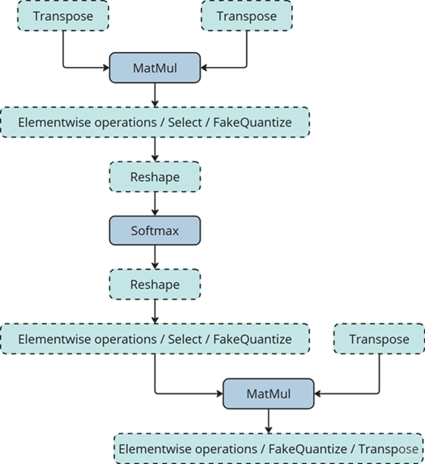
Note that SDPA has quadratic time and memory complexity with respect to sequence length. It means that by fusing SDPA-like patterns, Snippets significantly reduce memory consumption and accelerate transformer models, especially for large sequence lengths.

Snippets effectively optimized SDPA patterns but had a key limitation: they did not support dynamic shapes. In other words, input shapes must be known at the model compilation stage and can’t be changed in runtime. This limitation reduced the applicability of Snippets to many real-world scenarios where input shapes are not known in advance. While it is technically possible to JIT-compile a new binary for each unique set of input shapes, this approach introduces significant recompilation overheads, often negating the performance gains from SDPA fusion.

Fortunately, this static-shape limitation is not inherent to Snippets design. They can be modified to support dynamic shapes internally and generate shape-agnostic binaries. In this post, we discuss Snippets architecture and the challenges we faced during this dynamism enablement.

Architecture

The first step of the Snippets pipeline is called Tokenization. It is applied to an ov::Model, which represents OpenVINO Intermediate Representation (IR). It’s a standard IR in the OV Runtime you can read more about it here or here. The purpose of this stage is to identify parts of the initial model that can be lowered by Snippets efficiently. We are not going to discuss Tokenization in detail because this article is mostly focused on the dynamism implementation. A more in-depth description of the Tokenization process can be found in the Snippets design guide. The key takeaway for us here is that the subsequent lowering is performed on a part of the initial ov::Model. We will call this part Subgraph, and the Subgraph at first is also represented as an ov::Model.

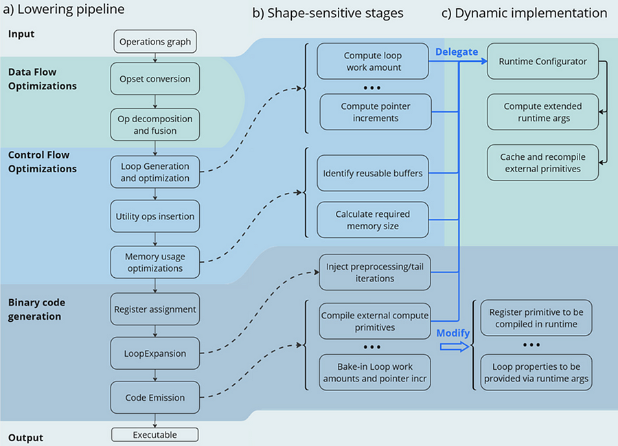
Now let’s have a look at the lowering pipeline, its schematic representation is shown on Fig.2a. As can be seen from the picture, the lowering process consists of three main phases: Data Flow Optimizations, Control Flow Optimizations and Binary Code Generation. Let’s briefly discuss each of them.

Lowering Pipeline

The first stage is the Data Flow optimizations. As we mentioned above, this stage’s input is a part of the initial model represented as an ov::Model. This representation is very convenient for high-level transformations such as opset conversion, operations’ fusion/decomposition and precision propagation. Here are some examples of the transformations performed on this stage:

1. ConvertPowerToPowerStatic — operation Power with scalar exponent input is converted to PowerStatic operation from the Snippets opset. The PowerStatic ops then use the values of the exponents to produce more optimal code.
2. FuseTransposeBrgemm — Transpose operations that can be executed in-place with Brgemm blocks are fused into the Brgemm operations.
3. PrecisionPropagation pass automatically inserts Converts operations between the operations that don’t natively support the desired execution precision.

The next stage of the lowering process is Control Flow optimizations (or simply CFOs). Note that the ov::Model is designed to primarily describe data flow, so is not very convenient for CFOs. Therefore, we had to develop our own IR (called Linear IR or simply LIR) that explicitly represents both control and data flows, you can read more about LIR here. So the ov::Model IR is converted to LIR before the start of the CFOs.

As you can see from the Fig.2a, the Control Flow optimization pipeline could roughly be divided into three main blocks. The first one is called Loop Generation and Optimization. This block includes all loop-related optimizations such as automatic generation of loops based on the input tensors’ dimensions, loop fusion and blocking loops generation.

The second block of Control Flow optimizations is called Utility Ops Insertion. We need this block of transformations here to insert utility operations that depend on loop control structures, specifically on their entry and exit points locations. For example, operations like Load, Store, MemoryBuffer, LoopBegin and LoopEnd are inserted during this stage.

The last step of CFO is the Memory Usage Optimizations block. These transformations determine required sizes of internal memory buffers, and analyze how much of that memory can be reused. A graph coloring algorithm is employed to minimize memory consumption.

Now all Control Flow optimizations are performed, and we are ready to proceed to the next stage of the lowering pipeline — Binary Code Generation (BCG). As one can see from Fig.2a, this stage consists of three substages. The first one is Register Assignment. We use a fairly standard approach here: calculate live intervals first and use the linear scan algorithm to assign abstract registers that are later mapped to physical ones.

The next BSG substage is Loop Expansion. To better understand its purpose, let’s switch gears for a second and think about loops in general. Sometimes it’s necessary to process the first or the last iteration of a loop in a special way. For example, to initialize a variable or to process blocking loops’ tails. The Loop Expansion pass unrolls these special iterations (usually the first or the last one) and explicitly injects them into the IR. This is needed to facilitate subsequent code emission.

The final step of the BCG stage is Code Emission. At this stage, every operation in our IR is mapped to a binary code emitter, which is then used to produce a piece of executable code. As a result, we produce an executable that performs calculations described by the initial input ov::Model.

Dynamic Shapes Support

Note that some stages of the lowering pipeline are inherently shape-sensitive, i.e. they rely on specific values of input shapes to perform optimizations. These stages are schematically depicted on the Fig. 2b.

As can be seen from the picture, shapes are used to determine loops’ work amounts and pointer increments that should be performed on every iteration. These parameters are later baked into the executable during Code Emission. Another example is Memory Usage Optimizations, since input shapes are needed to calculate memory consumption. Loop Expansion also relies on input shapes, since it needs to understand if tail processing is required for a particular loop. Note also that Snippets use compute primitives from third-party libraries, BRGEMM block from OneDNN for example. These primitives should as well be compiled with appropriate parameters that are also shape-sensitive.

One way to address these challenges is to rerun the lowering pipeline for every new set of input shapes, and to employ caching to avoid processing the same shapes twice. However, preliminary analysis indicated that this approach is too slow. Since this re-lowering needs to be performed in runtime, the performance benefit provided by Snippets is essentially eliminated by the recompilation overheads.

The performed experiments thus indicate that we can afford to run the whole lowering pipeline only once during the model compilation stage. Only some minor adjustments can be made at runtime. In other words, we need to remove all shape-sensitive logic from the lowering pipeline and perform the compilation without it. The remaining shape-sensitive transformations should be performed at runtime. Of course, we would also need to share this runtime context with the compiled shape-agnostic kernel. The idea behind this approach is schematically represented on Fig. 2c.

As one can see from the picture, all the shape-sensitive transformations are now performed by a new entity called Runtime Configurator. It’s probably easier to understand its purpose in some examples.

Imagine that we need to perform a unary operation get_result(X) on an input tensor X — for example, apply an activation function. To do this, we need to load some input data from memory into registers, perform the necessary computations and write the results back to memory. Of course this read-compute-write sequence should be done in a loop since we need to process the entire input tensor. These steps are described in more detail in Fig. 3 using pseudocode. Fig. 3a corresponds to a static kernel while Fig. 3b represents a dynamic one.

Let’s consider the static kernel as a starting point. As the first step, we need to load pointers to input and output memory blobs to general-purpose registers (or simply GPRs) denoted G_IN and G_OUT on the picture. Then we initialize another GPR that stores the loop work amount (G_WA). Note that the loop is used to traverse the input tensor, so the loop’s work amount is fixed because the tensor’s dimensions are also known at the BCG stage. The next six steps in the picture (3 to 8) are in the loop’s body.

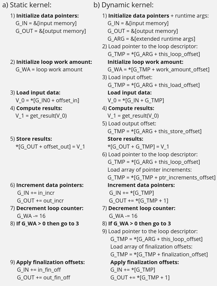
In step 3, we load input data into a vector register V_0, note that the appropriate pointer is already loaded to G_IN, and offset_in is fixed because the input tensor is static. Next, we apply our get_result function to the data in V_0 and place the result in a spare vector register V_1. Now we need to store V_1 back to memory, which is done on step 5. Note that offset_out is also known in the static case. This brings us almost to the end of the loop’s body, and the last few things we need to do are to increment data pointers (step 6), decrement loop counter (step 7), and jump to the beginning of the body, if needed (step 8).

Finally, we need to reset data pointers to their initial values after the loop is finished, which is done using finalization offsets on step 9. Note that this step could be omitted in our simplified example, but it’s often needed for more complicated use cases, such as when the data pointers are used by subsequent loops.

Now that we understand the static kernel, let’s consider the dynamic one, which is shown in Fig. 3b. Unsurprisingly, the dynamic kernel performs essentially the same steps as the static one, but with additional overhead due to loading shape-dependent parameters from the extended runtime arguments. Take step 1 as an example, we need to load not only memory pointers (to G_IN and G_OUT), but also a pointer to the runtime arguments prepared by the runtime configurator (to G_ARG).

Next, we need to load a pointer to the appropriate loop descriptor (a structure that stores loops’ parameters) to a temporary register G_TMP, and only then we can initialize the loop’s work amount register G_WA (step 2). Similarly, in order to load data to V_0, we need to load a runtime-calculated offset from the runtime arguments in step 3. The computations in step 4 are the same as in the static case, since they don’t depend on the input shapes. Storing the results to memory (step 5) requires reading a dynamic offset from the runtime arguments again. Next, we need to shift the data pointers, and again we have to load the increments from the corresponding loop descriptor in G_ARG because they are also shape-dependent, as the input tensor can be strided. The following two steps 7 and 8 are the same as in the static case, but the finalization offsets are also dynamic, so we have to load them from G_ARG yet again.

As one can see from Fig. 3, dynamic kernels incorporate additional overhead due to reading the extended runtime parameters provided by the runtime configurator. However, this overhead could be acceptable as long as the input tensor is large enough (Load/Store operations would take much longer than reading runtime arguments from L1) and the amount of computation is sufficient (get_results is much larger than the overhead). Let’s consider the performance of this design in the Results section to see if these conditions are met in practical use cases.

Results

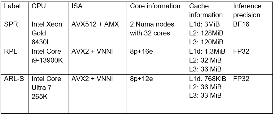
We selected three platforms to evaluate the dynamic pipeline’s performance in Snippets. These platforms represent different market segments: the Intel Core machine is designed for high-performance user and professional tasks. While the Intel Xeon is a good example of enterprise-level hardware often used in data centers and cloud computing applications. The information about the platforms is described in the table below:

As discussed in the Introduction, Snippets support various SDPA-like patterns which form the backbone of Transformer models. These models often work with input data of arbitrary size (for example, sequence length in NLP). Thus, dynamic shapes support in Snippets can efficiently accelerate many models based on Transformer architecture with dynamic inputs.

We selected 43 different Transformer-models from HuggingFace to measure how the enablement of dynamic pipeline in Snippets affects performance. The models were downloaded and converted to OpenVINO IRs using Optimum Intel. These models represent different domains and were designed to solve various tasks in natural language processing, text-to-image image generation and speech recognition (see full model list at the end of the article). What unifies all these models is that they all contain SDPA subgraph and thus can be accelerated by Snippets.

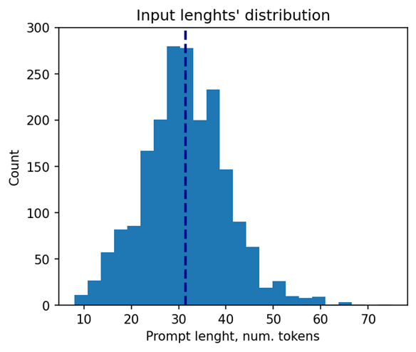
Let’s take a closer look at the selected models. The 37 models of them solve different tasks in natural language processing. Their performance was evaluated using a list of 2000 text sequences with different lengths, which also mimics the real-word scenario. The total processing time of all the sequences were measured in every experiment. Note that the text sequences were converted to model inputs using model-specific tokenizers prior to the benchmarking. The lengths’ distribution of the tokenized sequences is shown on Fig. 4. As can be seen from the picture, the distribution is close to normal with the mean length of 31 tokens.

The other 6 models of the selected model scope solve tasks in text-to-image image generation (Stable Diffusion) and speech recognition (Whisper). These models decompose into several smaller models after export to OpenVINO representation using Optimum Intel. Stable Diffusion topology is decomposed into Encoder, Diffuser and Decoder. The most interesting model here is Diffuser because it’s the one responsible for denoising of the latent image representation. This generation stage is repeated several times, so it is the most computationally intensive, which mostly effects on the generation time of the image. Whisper is also decomposed into Encoder and Decoder, which also contain SDPA patterns. The Encoder encodes the spectrogram from the feature extractor to form a sequence of encoder hidden states. Then, the decoder autoregressively predicts text tokens, conditional on both the previous tokens and the encoder hidden states. Currently, Snippets support efficient execution of SDPA only in Whisper Encoder, while Decoder is a subject for future support. To evaluate the inference performance of Stable Diffusion and Whisper models, we collect generation time of image/speech using LLM Benchmark from openvino.genai. This script provides a unified approach to estimate performance for GenAI workloads in OpenVINO.

Performance Improvements

Note that the main goal of these experiments is to estimate the impact of Snippets on the performance of the dynamic pipeline. To do that, we performed two series of experiments for every model. The first version of experiments is with disabled Snippets tokenization. In this case, all operations from the SDPA pattern are performed on the CPU plugin side as stand-alone operations. The second variant of experiments — with enabled Snippets tokenization. The relative difference between numbers collected on these two series of experiments is our performance metric — speedup, the higher the better. Firstly, let’s take a closer look at the resulting speedups for the BERT models which are depicted on Fig. 5.

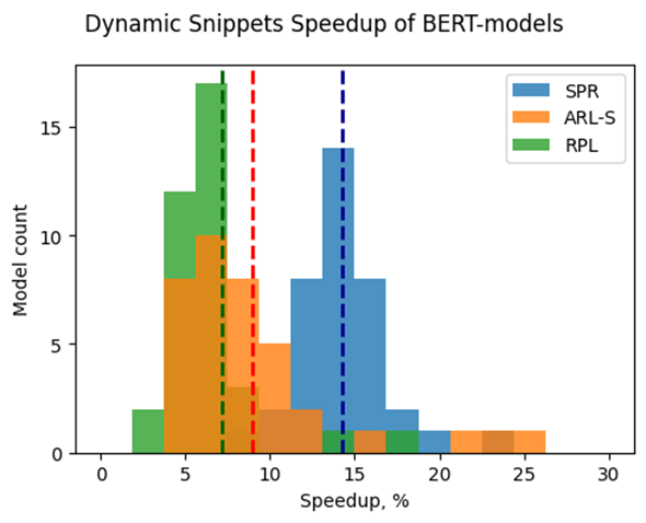
The speedups on RPL range from 3 to 18%, while on average the models are accelerated by 7%. The ARL-S speedups are somewhat higher and reach 20–25% for some models, the average acceleration factor is around 9%. The most affected platform is SPR, it has the highest average speedup of 15 %.

One can easily see from these numbers that both average and maximum speedups depend on the platform. To understand the reason for this variation, we should recall that the main optimizations delivered by Snippets are vertical fusion and tiling. These optimizations improve cache locality and reduce the memory access overheads. Note SPR has the largest caches among the examined platforms. It also uses BF16 precision that takes two times less space per data element compared to F32 used on ARL-S and RPL. Finally, SPR has AMX ISA extension that allows it to perform matrix multiplications much faster. As a result, SDPA execution was more memory bound on SPR, so this platform benefited the most from the Snippets enablement. At the same time, the model speedups on ARL-S and RPL are almost on the same level. These platforms use FP32 inference precision while SPR uses BF16, and they have less cache size than SPR.

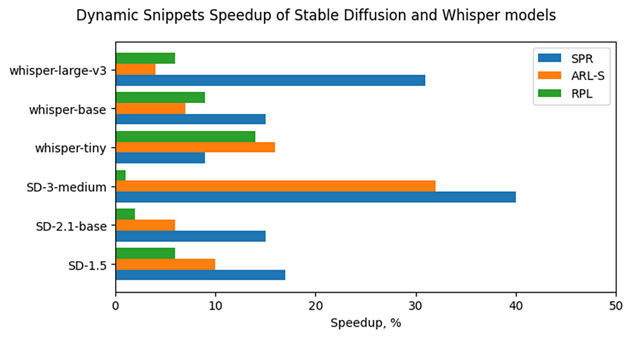
Now, let’s consider Stable Diffusion and Whisper topologies and compare their speedups with some of BERT-like models. As can be seen from the Fig. 6, the most accelerated Stable Diffusion topology is StableDiffusion-3-medium — almost 33% on ARL-S and 40% on SPR. The most accelerated model in this Stable Diffusion pipeline is Diffuser. This model has made a great contribution to speeding up the entire image generation time. The reason the Diffuser benefits more from Snippets enablement is that they use larger sequence lengths and embedding sizes. It means that their attention blocks process more data and are more memory constrained compared to BERT-like models. As a result, the Diffuser models in Stable Diffusion benefit more from the increased cache locality provided by Snippets. This effect is more pronounced on the SPR than on the ARL-S and RPL for the reasons discussed above (cache sizes, BF16, AMX).

The second most accelerated model is whisper-large-v3–30% on SPR. This model has more parameters than base and tiny models and process more Mel spectrogram frequency bins than they. It means that Encoder of whisper-large-v3 attention blocks processes more data, like Diffuser part of Stable Diffusion topologies. By the same reasons, whisper-large-v3 benefits more (increased cache locality provided by Snippets).

Memory Consumption Improvements

Another important improvement from Snippets using is reduction of memory consumption. Snippets use vertical fusion and various optimizations from Memory Usage Optimizations block (see the paragraph “Lowering Pipeline” in “Architecture” above for more details). Due to this fact, Subgraphs tokenized by Snippets consumes less memory than the same operations performed as stand-alone in CPU Plugin.

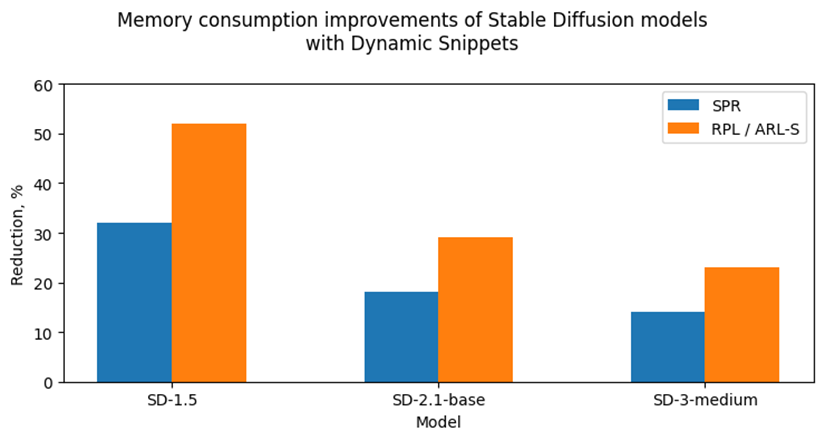
Let’s take a look at the Fig. 7 where we can see improvements in image generation memory consumption using Stable Diffusion pipelines from Snippets usage. As discussed above, the attention blocks in the Diffuser models from these pipelines process more data and consume more memory. Because of that, the greatest impact on memory consumption from using Snippets is seen on Stable Diffusion pipelines. For example, memory consumption of image generation is reduced by 25–50% on RPL and ARL-S platforms with FP32 inference precision and by 15–30% on SPR with BF16 inference precision.

Thus, one of the major improvements from using Snippets is memory consumption reduction. It allows extending the range of platforms which are capable to infer such memory-intensive models as Stable Diffusion.

Conclusion

Snippets is a JIT compiler used by OpenVINO to optimize performance-critical subgraphs. We briefly discussed Snippets’ lowering pipeline and the modifications made to enable dynamism support. After these changes, Snippets generate shape-agnostic kernels that can be used for various input shapes without recompilation.

This design was tested on realistic use cases across several platforms. As a result, we demonstrate that Snippets can accelerate BERT-like models by up to 25%, Stable Diffusion and Whisper pipelines up to 40%. Additionally, Snippets can significantly reduce memory consumption by several tens of percent. Notably, these improvements result from more optimal hardware utilization, so the models’ accuracy remains unaffected.

References

Model list can be found here: https://gist.github.com/a-sidorova/2c2aa584922389138e5ccbad0e0c773b

Intel Xeon Gold 6430L: https://www.intel.com/content/www/us/en/products/sku/231737/intel-xeon-gold-6430-processor-60m-cache-2-10-ghz/specifications.html

Intel Core i9-13900K: https://www.intel.com/content/www/us/en/products/sku/230496/intel-core-i913900k-processor-36m-cache-up-to-5-80-ghz/specifications.html

Intel Core Ultra 7 265K: https://www.intel.com/content/www/us/en/products/sku/241063/intel-core-ultra-7-processor-265k-30m-cache-up-to-5-50-ghz/specifications.html

Notices & Disclaimers

Performance varies by use, configuration, and other factors. Learn more on the Performance Index site.

No product or component can be absolutely secure. Your costs and results may vary. Intel technologies may require enabled hardware, software or service activation.

© Intel Corporation. Intel, the Intel logo, and other Intel marks are trademarks of Intel Corporation or its subsidiaries.

‍

OpenVINO and OneDNN

OpenVINO™ is a framework designed to accelerate deep-learning models from DL frameworks like Tensorflow or Pytorch. By using OpenVINO, developers can directly deploy inference application without reconstructing the model by low-level API. It consists of various components, and for running inference on a GPU, a key component is the highly optimized deep-learning kernels, such as convolution, pooling, or matrix multiplication.

On the other hand, Intel® oneAPI Deep Neural Network Library (oneDNN), is a library that provides basic deep-learning building blocks, mainly kernels. It differs from OpenVINO in a way that OneDNN provides APIs for running deep-learning nodes like convolution, but not for running deep-learning models such as Resnet-50.

OpenVINO utilizes OneDNN GPU kernels for discrete GPUs, in addition to its own GPU kernels. It is to accelerate compute-intensive workloads to an extreme level on discrete GPUs. While OpenVINO already includes highly-optimized and mature deep-learning kernels for integrated GPUs, discrete GPUs include a new hardware block called a systolic array, which accelerates compute-intensive kernels. OneDNN provides these kernels with systolic array usage.

If you want to learn more about the systolic array and the advancements in discrete GPUs, please refer to this article.

How does OneDNN accelerates DL workloads for OpenVINO?

When you load deep-learning models in OpenVINO, they go through multiple stages called graph compilation. The purpose of graph compilation is to create the "execution plan" for the model on the target hardware.

During graph compilation, OpenVINO GPU plugin checks the target hardware to determine whether it has a systolic array or not. If the hardware has a systolic array(which means you have a discrete GPU like Arc, Flex, or GPU Max series), OpenVINO compiles the model so that compute-intensive layers are processed using OneDNN kernels.

OpenVINO kernels and OneDNN kernels use a single OpenCL context and shared buffers, eliminating the overhead of buffer-copying. For example, OneDNN layer computes a layers and fills a buffer, which then may be read by OpenVINO kernels because both kernels run in a single OpenCL context.

You may wonder why only some of the layers are processed by OneDNN while others are still processed by OpenVINO kernels. This is due to the variety of required kernels. OneDNN includes only certain key kernels for deep learning while OpenVINO contains many kernels to cover a wide range of models.

OneDNN is statically linked to OpenVINO GPU Plugin, which is why you cannot find the OneDNN library from released OpenVINO binary. The dynamic library of OpenVINO GPU Plugin includes OneDNN.

The GPU plugin and the CPU plugin have separate versions of OneDNN. To reduce the compiled binary size, the OpenVINO GPU plugin contains only the GPU kernels of OneDNN, and the OpenVINO CPU plugin contains only the CPU kernels of OneDNN.

Hands-on Tips and FAQs

What should an application developer do to take advantage of OneDNN?

If the hardware supports a systolic array and the model has layers that can be accelerated by OneDNN, it will be accelerated automatically without any action required from application developers.

How can I determine whether OneDNN kernels are being used or not?

You can check the OneDNN verbose log or the executed kernel names.

Set `ONEDNN_VERBOSE=1` to see the OneDNN verbose log. Then you will see a bunch of OneDNN kernel execution log, which means that OneDNN kernels are properly executed. Each execution of OneDNN kernel will print a line. If all kernels are executed without OneDNN, you will not see any of such log line.

$ ONEDNN_VERBOSE=1 ./benchmark_app -m resnet-50.xml -d GPU --niter 1
[Step 1/11] Parsing and validating input arguments
[ INFO ] Parsing input parameters
[Step 2/11] Loading OpenVINO Runtime
...
onednn_verbose,exec,gpu,convolution,jit:ir,forward_inference,src_s8::blocked:abcd:f0 wei_s8:p:blocked:AcdB8a4b:f0 bia_f32::blocked:a:f0 dst_u8::blocked:aBcd32b:f0,attr-post-ops:binary_mul:f32:2 ,alg:convolution_direct,mb1_ic3oc64_ih224oh112kh7sh2dh0ph3_iw224ow112kw7sw2dw0pw3,0.319092
onednn_verbose,exec,gpu,pooling,ocl:gen9,forward_inference,src_u8::blocked:aBcd32b:f0 dst_u8::blocked:aBcd32b:f0 ws_undef::undef::,,alg:pooling_max,mb1ic64_ih112oh56kh3sh2dh0ph0_iw112ow56kw3sw2dw0pw0,0.0788574
onednn_verbose,exec,gpu,convolution,jit:ir,forward_inference,src_u8::blocked:aBcd32b:f0 wei_s8::blocked:ABcd8b8a4b:f0 bia_f32::blocked:a:f0 dst_u8::blocked:aBcd32b:f0,attr-post-ops:binary_mul:f32:2 ,alg:convolution_direct,mb1_ic64oc64_ih56oh56kh1sh1dh0ph0_iw56ow56kw1sw1dw0pw0,0.199951
onednn_verbose,exec,gpu,convolution,jit:ir,forward_inference,src_u8::blocked:aBcd32b:f0 wei_s8::blocked:ABcd8b8a4b:f0 bia_f32::blocked:a:f0 dst_u8::blocked:aBcd32b:f0,attr-post-ops:binary_mul:f32:2 ,alg:convolution_direct,mb1_ic64oc64_ih56oh56kh3sh1dh0ph1_iw56ow56kw3sw1dw0pw1,0.111084
onednn_verbose,exec,gpu,convolution,jit:ir,forward_inference,src_u8::blocked:aBcd32b:f0 wei_s8::blocked:ABcd8b8a4b:f0 bia_f32::blocked:a:f0 dst_s8::blocked:aBcd32b:f0,attr-post-ops:binary_mul:f32:2+binary_add:f32:2 ,alg:convolution_direct,mb1_ic64oc256_ih56oh56kh1sh1dh0ph0_iw56ow56kw1sw1dw0pw0,0.0688477
onednn_verbose,exec,gpu,convolution,jit:ir,forward_inference,src_u8::blocked:aBcd32b:f0 wei_s8::blocked:ABcd8b8a4b:f0 bia_f32::blocked:a:f0 dst_u8::blocked:aBcd32b:f0,attr-post-ops:binary_mul:f32:2+binary_add:f32:2+eltwise_round+eltwise_linear:1.77854:-227.654+eltwise_clip:-227.654:225.875+sum:1:0:s8+eltwise_linear:1.59738 ,alg:convolution_direct,mb1_ic64oc256_ih56oh56kh1sh1dh0ph0_iw56ow56kw1sw1dw0pw0,0.0771484
onednn_verbose,exec,gpu,convolution,jit:ir,forward_inference,src_u8::blocked:aBcd32b:f0 wei_s8::blocked:ABcd8b8a4b:f0 bia_f32::blocked:a:f0 dst_u8::blocked:aBcd32b:f0,attr-post-ops:binary_mul:f32:2 ,alg:convolution_direct,mb1_ic256oc64_ih56oh56kh1sh1dh0ph0_iw56ow56kw1sw1dw0pw0,0.0678711
onednn_verbose,exec,gpu,convolution,jit:ir,forward_inference,src_u8::blocked:aBcd32b:f0 wei_s8::blocked:ABcd8b8a4b:f0 bia_f32::blocked:a:f0 dst_u8::blocked:aBcd32b:f0,attr-post-ops:binary_mul:f32:2 ,alg:convolution_direct,mb1_ic64oc64_ih56oh56kh3sh1dh0ph1_iw56ow56kw3sw1dw0pw1,0.108154
...

Alternatively, you can check the kernel names from performance counter option from benchmark_app. (--pc)

OneDNN layers include colon in the `execType` field as shown below. In this case, convolutions are handled by OneDNN jit:ir kernels. MaxPool is also handled by OneDNN kernel that is implemented with OpenCL.(and in this case, the systolic array is not used)

$ ./benchmark_app -m resnet-50.xml -d GPU --niter 1 -nstreams 1 --nireq 1 --hint none --pc | grep -v OPTIMIZED_OUT
[Step 1/11] Parsing and validating input arguments
...
input                EXECUTED             layerType: Parameter            execType:
wait_for_events__u8  realTime (ms): 0.001      cpuTime (ms): 0.000      
resnet_v1_50/po...   EXECUTED             layerType: MaxPool              execType: ocl:gen9__u8         realTime (ms): 0.114      cpuTime (ms): 0.000      
resnet_v1_50/bl...   EXECUTED             layerType: MaxPool              execType: ocl:gen9__u8         realTime (ms): 0.070      cpuTime (ms): 0.000      
resnet_v1_50/bl...   EXECUTED             layerType: MaxPool              execType: ocl:gen9__u8         realTime (ms): 0.065      cpuTime (ms): 0.000      
resnet_v1_50/bl...   EXECUTED             layerType: MaxPool              execType: ocl:ref__u8          realTime (ms): 0.061      cpuTime (ms): 0.000      
resnet_v1_50/pool5   EXECUTED             layerType: ReduceMean           execType: ocl:combined__u8     realTime (ms): 0.077      cpuTime (ms): 0.000      
resnet_v1_50/Sp...   EXECUTED             layerType: Result               execType: reorder_data_fast_b1__f32 realTime (ms): 0.014      cpuTime (ms): 0.003      
resnet_v1_50/co...   EXECUTED             layerType: FakeQuantize         execType: quantize_gpu_scale_shift_opt__i8 realTime (ms): 0.042      cpuTime (ms): 0.017      
resnet_v1_50/co...   EXECUTED             layerType: Convolution          execType: jit:ir__i8           realTime (ms): 0.524      cpuTime (ms): 0.000      
resnet_v1_50/bl...   EXECUTED             layerType: Convolution          execType: jit:ir__u8           realTime (ms): 0.129      cpuTime (ms): 0.000      
resnet_v1_50/bl...   EXECUTED             layerType: Convolution          execType: jit:ir__u8           realTime (ms): 0.123      cpuTime (ms): 0.000      
...

Can we run networks without Onednn on discrete GPU?

It is not supported out-of-box and it is not recommended to do so because systolic array will not be used and the performance will be very different.
If you want to try without OneDNN still, you can follow this documentation and use `OV_GPU_DisableOnednn`.

How to know whether my GPU will be accelerated with OneDNN(or it has systolic array or not)?

You can use hello_query_device from OpenVINO sample app to check whether it has `GPU_HW_MATMUL` in `OPTIMIZATION_CAPABILITIES`.

$ ./hello_query_device 
[ INFO ] Available devices: 
[ INFO ] GPU
[ INFO ]        SUPPORTED_PROPERTIES: 
...
[ INFO ]                Immutable: FULL_DEVICE_NAME : Intel(R) Arc(TM) A770 Graphics (dGPU)
...
[ INFO ]                Immutable: OPTIMIZATION_CAPABILITIES : FP32 BIN FP16 INT8 GPU_HW_MATMUL EXPORT_IMPORT

How to check the version of OneDNN?

You can set `ONEDNN_VERBOSE=1` to check see the verbose log. Below, you can see that OneDNN version is v3.1 as an example. (OnnDNN 3.1 was used for OpenVINO 23.0 release)
Please note that it is shown only when OneDNN is actually used in the target hardware. If the model is not accelerated through OneDNN, OneDNN version will not be shown.

$ ONEDNN_VERBOSE=1 ./benchmark_app -m resnet-50.xml -d GPU --niter 1
[Step 1/11] Parsing and validating input arguments
[ INFO ] Parsing input parameters
[Step 2/11] Loading OpenVINO Runtime
...
[Step 7/11] Loading the model to the device
onednn_verbose,info,oneDNN v3.1.0 (commit f27dedbfc093f51032a4580198bb80579440dc15)
onednn_verbose,info,gpu,runtime:OpenCL
onednn_verbose,info,gpu,engine,0,name:Intel(R) Arc(TM) A770 Graphics,driver_version:23.17.26241,binary_kernels:enabled

Is it possible to try different OneDNN version?

As it is statically linked, you cannot try different OneDNN version from single OpenVINO version. It is also not recommended to build OpenVINO with different OneDNN version than it is originally built because we do not guarantee that it works properly.

How to profile OneDNN execution time?

Profiling is also integrated to OpenVINO. So you can use profiling feature of OpenVINO, such as --pc and --pcsort option from benchmark_app. However, it includes some additional overhead for OneDNN and it may report higher execution time than actual time especially for small layers. More reliable method is to use DevicePerformanceTiming with opencl-intercept-layers.

‍

‍

Introduction

OpenVINO is an open-source toolkit for optimization and deployment of AI inference. OpenVINO results in more efficient inference of deep learning models at the edge or in data centers. OpenVINO compiles models to run on many different devices, meaning you will have the flexibility to write code once and deploy your model across CPUs, GPUs, VPUs and other accelerators.  

The new family of Intel discrete GPUs are not just for gaming, they can also run AI at the edge or on servers. Use this guide to install drivers and setup your system before using OpenVINO for GPU-based inference.

‍

OpenVINO and GPU Compatibility

To get the best possible performance, it’s important to properly set up and install the current GPU drivers on your system. Below, I provide some recommendations for installing drivers on Windows and Ubuntu. This article was tested on Intel® Arc™ graphics and Intel® Data Center GPU Flex Series on systems with Ubuntu 22.04 LTS and Windows 11. To use the OpenVINO™ GPU plugin and offload inference to Intel® GPU, the Intel® Graphics Driver must be properly configured on your system.  

‍

Recommended Configuration for Ubuntu 22.04 LTS

The driver for Ubuntu 22.04 works out of the box with Kernel 5.15.0-57. However, if you upgraded/downgraded your kernel or upgraded from Ubuntu 20.04 LTS to 22.04, I suggest updating the kernel version to linux-image-5.19.0-43-generic.  

After updating the kernel, check for the latest driver release. I updated my Ubuntu machine to version 23.13.26032.30, which was the latest version at the time of publishing this article, however OpenVINO could be run on discrete GPU with older or newer driver versions.  

NOTE: If you upgraded Ubuntu 20.04 to 22.04, please verify your kernel version `uname –r` before updating the driver.  

‍

Recommended Configuration for Windows 11

Many driver versions are available for Windows. To run AI workloads, I suggest using the latest beta driver.

‍

Getting Help

Even if you are using the latest available driver, you should always check if your AI models are running properly and generating the expected results. If you discover a bug for a particular model or failure to run a specific model, please file an issue on GitHub. Before reporting an issue, please check whether using the latest Beta version of the driver and latest version of OpenVINO solves the issue.  

NOTE: Always refer to the official GPU driver documentation when setting up your system. This blog provides additional recommendations for the best results when using OpenVINO but it is not a replacement for documentation.

‍

Conclusion

Checking the system requirements in Ubuntu 22.04 LTS and Windows 11 resolves some issues running Generative AI models like Stable Diffusion with OpenVINO on discrete GPUs. These updates prevent crashes and compilation errors or poor performance with Stable Diffusion. I suggest testing your AI models with the new driver installation, as it will likely improve the performance of your application. Try out this Stable Diffusion notebook for testing purposes.  

Resources

https://github.com/intel/compute-runtime/

https://www.intel.com/content/www/us/en/products/docs/discrete-gpus/arc/software/drivers.html

https://www.intel.com/content/www/us/en/download/729157/intel-arc-iris-xe-graphics-beta-windows.html

https://docs.openvino.ai/2023.0/openvino_docs_OV_UG_supported_plugins_GPU.html  

https://github.com/openvinotoolkit/openvino_notebooks/tree/main/notebooks/108-gpu-device  

OpenVINO™ is a toolkit that enables developers to deploy pre-trained deep learning models through a C++ or Python inference engine API. The latest OpenVINO™ has enabled the PaddlePaddle quantized model, which helps accelerate their deployment.

From floating-point model to quantized model in PaddlePaddle

Baidu releases a toolkit for PaddlePaddle model compression, named PaddleSlim. The quantization is a technique in PaddleSlim, which reduces redundancy by reducing full precision data to a fixed number so as to reduce model calculation complexity and improve model inference performance. To achieve quantization, PaddleSlim takes the following steps.

1. Insert the quantize_linear and dequantize_linear nodes into the floating-point model.
2. Calculate the scale and zero_point in each layer during the calibration process.
3. Convert and export the floating-point model to quantized model according to the quantization parameters.

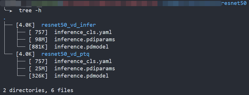
As the Figure1 shows, Compared to the floating-point model, the size of the quantized model is reduced by about 75%.

Enable PaddlePaddle quantized model in OpenVINO™

As the Figure2.1 shows, paired quantize_linear and dequantize_linear nodes appear intermittently in the model.

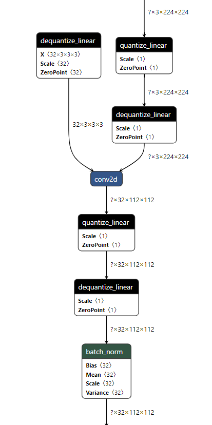
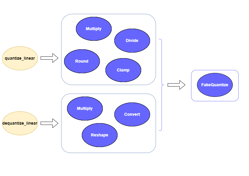
In order to enable PaddlePaddle quantized model, both quantize_linear and dequantize_linear nodes should be mapped first. And then, quantize_linear and dequantize_linear pattern scan be fused into FakeQuantize nodes and OpenVINO™ transformation mechanism will simplify and optimize the model graph in the quantization mode.

To check the kernel execution function, just profile and dump the execution progress, you can use benchmark_app as an example. The benchmark_app provides the option"-pc", which is used to report the performance counters information.

• To report the performance counters information of PaddlePaddle resnet50 float model, we can run the command line:

./benchmark_app -m resnet50_vd_infer/inference.pdmodel -data_shape "[1,3,224,224]"-pc -pcsort sort

• To report the performance counters information of PaddlePaddle resnet50 quantized model, we can run the command line:

./benchmark_app -m resnet50_vd_ptq/inference.pdmodel -data_shape "[1,3,224,224]"-pc -pcsort sort

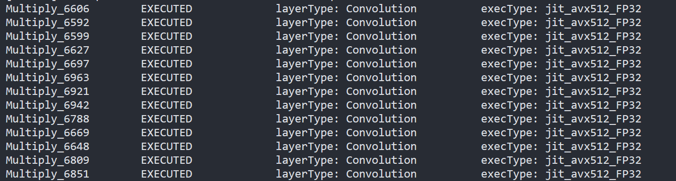
By comparing the Figure2.3 and Figure2.4, we can easily find that the hotpot layers of PaddlePaddle quantized model are dispatched to integer ISA implementation, which can accelerate the execution.

Accuracy

We compare the accuracy between resnet50 floating-point model and post training quantization(PaddleSlim PTQ) model. The accuracy of PaddlePaddle quantized model only decreases slightly, which is expected.

Performance

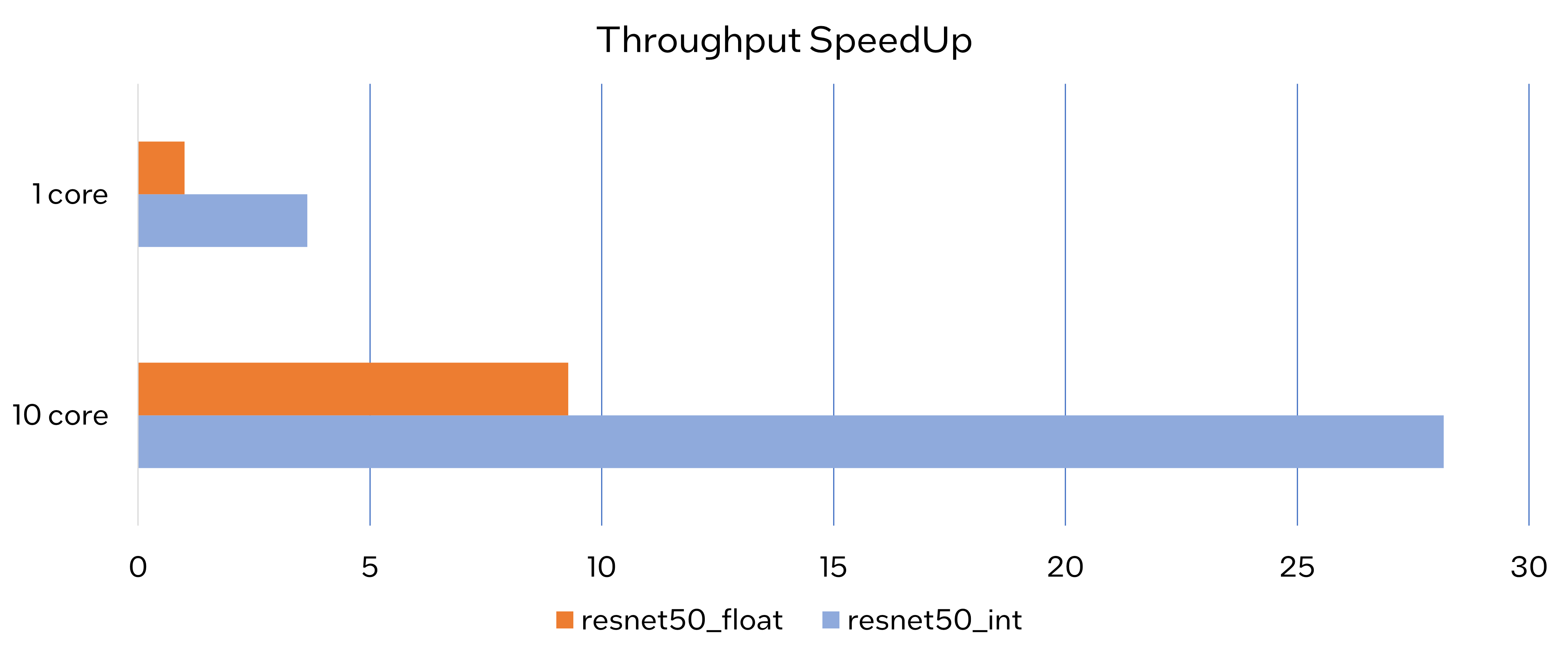
Throughput Speedup

The throughput of PaddlePaddle quantized resnet50 model can improve >3x.

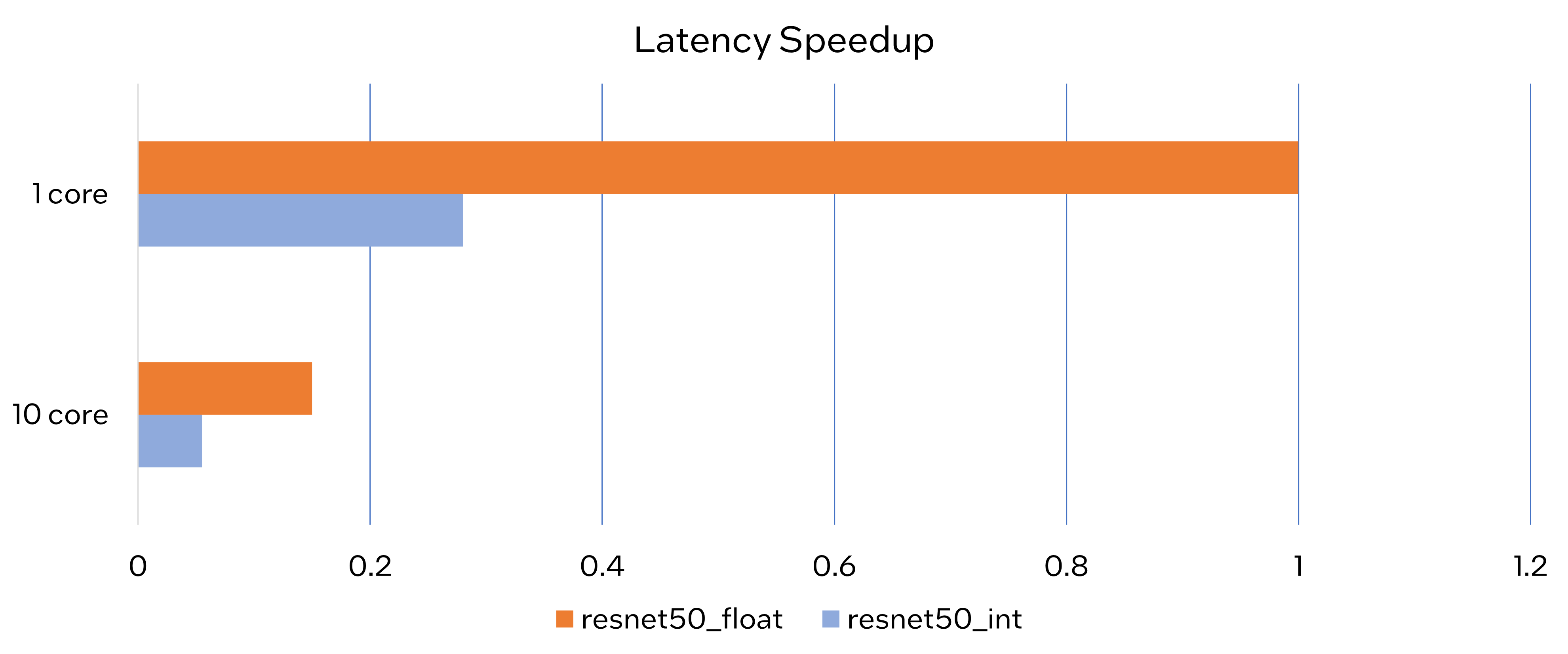
Latency Speedup

The latency of PaddlePaddle quantized resnet50 model can reduce about 70%.

Conclusion

In this article, we elaborated the PaddlePaddle quantized model in OpenVINO™ and profiled the accuracy and performance. By enabling the PaddlePaddle quantized model in OpenVINO™, customers can accelerate both throughput and latency of deployment easily.

Notices & Disclaimers

1. The accuracy data is collected based on 50000 images of val dataset in ILSVRC2012.
2. The throughput performance data is collected by benchmark_app with data_shape "[1,3,224,224]" and hint throughput.
3. The latency performance data is collected by benchmark_app with data_shape "[1,3,224,224]" and hint latency.
4. The machine is Intel® Xeon® Gold 6346 CPU @3.10GHz.
5. PaddlePaddle quantized model can be achieve at https://github.com/PaddlePaddle/FastDeploy/blob/develop/docs/en/quantize.md.

Authors: Mingyu Kim, Vladimir Paramuzov, Nico Galoppo

Intel’s newest GPUs, such as Intel® Data Center GPU Flex Series, and Intel® Arc™ GPU, introduce a range of new hardware features that benefit AI workloads. Starting with the 2022.3 release, OpenVINO™ can take advantage of two newly introduced hardware features: XMX (Xe Matrix Extension) and parallel stream execution. This article explains what those features are and how you can check whether they are enabled in your environment. We also show how to benefit from them with OpenVINO, and the performance impact of doing so.

What is XMX (Xe Matrix Extension)?

XMX is a hardware acceleration for matrix multiplication on the newest Intel™ GPUs. Given the same number of Xe Cores, XMX technology provides 4-8x more multiplication capacity at the same precision [1]. OpenVINO, powered by OneDNN, can take advantage of XMX hardware by accelerating int8 and fp16 inference. It brings performance gains in compute-intensive deep learning primitives such as convolution and matrix multiplication.

Under the hood, XMX is a well-known hardware architecture called a systolic array. Systolic arrays increase computational capacity without increasing memory (or register) access. The magic happens by pipelining multiple computations with a single data access, as opposed to the traditional fetch-compute-store pipeline. It is implemented by connecting multiple computation nodes in series. Data is fed into the front, goes through several steps of multiplication-add, and finally is stored back to memory.

How to check whether you have XMX?

You can check whether your GPU hardware (and software stack) supports XMX with OpenVINO™’s hello_query_device sample. When you run the sample application, it lists all detected inference devices along with its properties. You can check for XMX support by looking at the OPTIMIZATION_CAPABILITIES property and checking for the GPU_HW_MATMUL value.

In the listing below you can see that our system has two GPU devices for inference, and only GPU.1 has XMX support.

$ ./hello_query_device
[ INFO ] GPU.0
[ INFO ]        SUPPORTED_PROPERTIES: 
[ INFO ]                Immutable: OPTIMIZATION_CAPABILITIES : FP32 BIN FP16 INT8      
# XMX is not supported
[ INFO ] GPU.1
[ INFO ]        SUPPORTED_PROPERTIES: 
[ INFO ]                Immutable: OPTIMIZATION_CAPABILITIES : FP32 BIN FP16 INT8 GPU_HW_MATMUL    
# XMX is supported

‍

As mentioned, XMX provides a way to get significantly more compute capacity on a GPU. The next feature doesn’t provide more capacity, but it allows ways to use that capacity more efficiently.

What is parallel execution of multiple streams?

Another improvement of Intel®’s discrete GPUs is to process multiple compute streams in parallel. Certain deep learning inference workloads are too small to fill all hardware compute resources of a given GPU. In such a case it is beneficial to run multiple compute streams (or inference requests) in parallel, such that the GPU hardware has more work to process at any given point in time. With parallel execution of multiple streams, Intel GPUs can increase hardware efficiency.

How to check for parallel execution support?

As of the OpenVINO 2022.3 release, there is only an indirect way to query how many streams your GPU can process in parallel. In the next release it will be possible to query the range of streams using the ov::range_for_streams property query and the hello_query_device_sample. Meanwhile, one can use the benchmark_app to report the default number of streams (NUM_STREAMS). If the GPU does not support parallel stream execution, NUM_STREAMS will be 2. If the GPU does support it, NUM_STREAMS will be larger than 2. The benchmark_app log below shows that GPU.1 supports 4-stream parallel execution.

$ ./benchmark_app -d GPU.0 -m resnet-50.xml -t 1 --hint none
[ INFO ]   NUM_STREAMS: 2      # Single-stream execution is supported
…
$ ./benchmark_app -d GPU.1 -m resnet-50.xml -t 1 --hint none
[ INFO ]   NUM_STREAMS: 4      # 4-stream execution is supported
…

‍

However, it depends on application usage

Parallel stream execution can bring significant performance benefit, but only when used appropriately by the application. It will bring good performance gain if the application can run multiple independent inference requests in parallel, whether from single process or multiple processes. On the other hand, if there is no opportunity for parallel execution of multiple inference requests, then there is no gain to be had from multi-stream hardware execution.

Demonstration of performance tuning through benchmark_app

DISCLAIMER: The performance may vary depending on the system and usage.

OpenVINO benchmark_app is a very handy tool to analyze performance in various conditions. Here we’ll show the performance trend for an Intel® discrete GPU with XMX and four parallel hardware execution streams.

The performance was measured on a pre-production version of the Intel® Arc™ A770 Limited Edition GPU with 16 GiB of memory. The host system is a 12th Gen Intel(R) Core(TM) i9-12900K with 64GiB of RAM (4 DDR4-2667 modules) running Ubuntu OS 20.04.5 LTS with Linux kernel 5.15.47.

Performance comparison with high-level performance hints

Even though all supported devices in OpenVINO™ offer low-level performance settings, utilizing them is not recommended outside of very few cases. The preferred way to configure performance in OpenVINO Runtime is using performance hints. This is a future-proof solution fully compatible with the automatic device selection inference mode and designed with portability in mind.

OpenVINO benchmark_app exposes the high-level performance hints with the performance hint option for easy configuration of best latency and throughput. In short, latency mode picks the optimal configuration for low latency with the cost of low throughput, and throughput mode picks the optimal configuration for high throughput with the cost of high latency.

The table below shows throughput for various combinations of execution configuration for resnet-50.

‍

Throughput mode is achieving much higher FPS compared to latency mode because inference happens with higher batch size and parallel stream execution.  You can also see that, in throughput mode, the throughput with fp16 is 5.4x higher than with fp32 due to the use of XMX.

In the experiments below we manually explore different configurations of the performance parameters for demonstration purposes; It is generally not recommended to tune manually. Once the optimal parameters are known, they can be applied in production.

Performance gain from XMX

Performance gain from XMX can be observed by comparing int8/fp16 against fp32 performance because OpenVINO does not provide an option to turn XMX off. Since fp32 computations are not executed by the XMX hardware pipe, but rather by the less efficient fetch-compute-store pipe, you can see that the performance gap between fp32 and fp16 is much larger than the expected factor of two.

We choose a batch size of 64 to demonstrate the best case performance gain. When the batch size is small, the performance difference is not always as prominent since the workload could become too small for the GPU.

$ ./benchmark_app -d GPU.1 -m resnet-50-fp.xml -t 10 --hint none --nstreams 4 -b 64 --infer_precision f32 | grep Throughput
[ INFO ] Throughput:          1076.22 FPS 
$ ./benchmark_app -d GPU.1 -m resnet-50-fp.xml -t 10 --hint none --nstreams 4 -b 64 --infer_precision f16 | grep Throughput
[ INFO ] Throughput:          5915.62 FPS
$ ./benchmark_app -d GPU.1 -m resnet-50-int8.xml -t 10 --hint none --nstreams 4 -b 64 | grep Throughput
[ INFO ] Throughput:          12270.12 FPS

‍

As you can see from the execution log, fp16 runs ~5.49x faster than fp32. Int8 throughput is ~2.07x higher than fp16. The difference between fp16 and fp32 is due to fp16 acceleration from XMX while fp32 is not using XMX. The performance gain of int8 over fp16 is 2.07x because both are accelerated with XMX.

Performance gain from parallel stream execution

You can see from the log below that performance goes up as we have more streams up to 4. It is because the GPU can handle 4 streams in parallel.

$./benchmark_app -d GPU.1 -m resnet-50-int8.xml -t 10 --hint none --nstreams 1 -b 64 | grep Throughput
[ INFO ] Throughput:          8593.92 FPS
$./benchmark_app -d GPU.1 -m resnet-50-int8.xml -t 10 --hint none --nstreams 2 -b 64 | grep Throughput
[ INFO ] Throughput:          10610.98 FPS
$./benchmark_app -d GPU.1 -m resnet-50-int8.xml -t 10 --hint none --nstreams 4 -b 64 | grep Throughput
[ INFO ] Throughput:          12246.29 FPS
$./benchmark_app -d GPU.1 -m resnet-50-int8.xml -t 10 --hint none --nstreams 8 -b 64 | grep Throughput
[ INFO ] Throughput:          12150.30 FPS

‍

Note that if the inference workload is large enough, more streams might not bring much or any performance gain. For example, when increasing the batch size, throughput may saturate earlier than at 4 streams.

How to take advantage the improvements in your application

For XMX, all you need to do is run your int8 or fp16 model with the OpenVINO™ Runtime version 2022.3 or above. If the model is fp32(single precision), it will not be accelerated by XMX. To quantize a model and create an OpenVINO int8 IR, please refer to Quantizing Models Post-training. To create an OpenVINO fp16 IR from a fp32 floating-point model, please refer to Compressing a Model to FP16 page.

For parallel stream execution, you can set throughput hint as described in Optimizing for Throughput. It will automatically set the number of parallel streams with best number.

Conclusion

In this article, we introduced two key features of Intel®’s discrete GPUs: XMX and parallel stream execution. Most int8/fp16 deep learning networks can benefit from the XMX engine with no additional configuration. When properly configured by the application, parallel stream execution can bring significant performance gains too!

‍

[1] In the Xe-HPG architecture, the XMX delivers 256 INT8 ops per clock (DPAS), while the (non-systolic) Xe Core vector engine delivers 64 INT8 ops per clock – a 4x throughput increase [reference]. In the Xe-HPC architecture, the XMX systolic array depth has been increased to 8 and delivers 4096 FP16 ops per clock, while the (non-systolic) Xe Core vector engine delivers 512 FP16 ops per clock – a 8x throughput increase [reference].

‍

Notices & Disclaimers

​Performance varies by use, configuration and other factors. Learn more at www.Intel.com/PerformanceIndex​​.

Performance results are based on testing as of dates shown in configurations and may not reflect all publicly available ​updates.  See backup for configuration details.  No product or component can be absolutely secure.​​

​​​​See backup for configuration details.  For more complete information about performance and benchmark results, visit www.intel.com/benchmarks

© Intel Corporation.  Intel, the Intel logo, and other Intel marks are trademarks of Intel Corporation or its subsidiaries.  Other names and brands may be claimed as the property of others​.​​

Starting with the 2022.3 release, OpenVINO Model Server (OVMS) provides a C-API that allows OVMS to be linked directly into a C/C++ application as a dynamic library. Existing AI applications can leverage serving functionalities while running inference locally without networking latency overhead.  

The ability to bypass gRPC/REST endpoints and send input data directly from in-process memory creates new opportunities to use OpenVINO locally while maintaining the benefits of model serving. For example, we can combine the benefits of using OpenVINO Runtime with model configuration, version management and support for both local and cloud model storage.

‍

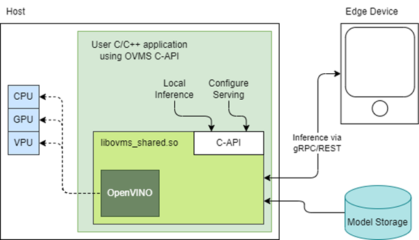
OpenVINO Model Server is typically started as a separate process or run in a container where the client application communicates over a network connection. Now, as you can see above, it is possible to link the model server as a shared library inside the client application and use the internal C API to execute internal inference methods.

We demonstrate the concept in a simple example below and show the impact on latency.

‍

Example C-API Usage

NOTE: complete end to end inference demonstration via C-API with example app can be found here: https://docs.openvino.ai/latest/ovms_demo_capi_inference_demo.html  

To start using the Model Server C-API, we need to prepare a model and configuration file. Download an example dummy model from our GitHub repo and prepare a config.json file to serve this model. “Dummy” model adds value 1 to all numbers inside an input.

‍

Download Model

wget https://github.com/openvinotoolkit/model_server/raw/main/src/test/dummy/1/dummy.{xml,bin} -P models/dummy/1

‍

Create Config File

{ 
    "model_config_list": [ 
        {"config": { 
                "name": "dummy", 
                "base_path": "./models/dummy"}} 
    ] 
} 

‍

Get libovms_shared.so

Next, download and unpack the OVMS library. The library can be obtained from GitHub release page. There are 2 packages – one for Ubuntu 20 and one for RedHat 8.7. There is also documentation showing how to build the library from source. For purpose of this demo, we will use the Ubuntu version:

wget https://github.com/openvinotoolkit/model_server/releases/download/v2022.3/ovms_ubuntu.tar.gz && tar -xvf ovms_ubuntu.tar.gz

‍

Start Server

To start the server, use ServerStartFromConfigurationFile. There are many options, all of which are documented in the header file. Let’s launch the server with configuration file and optional log level error:

OVMS_ServerSettings* serverSettings; 
OVMS_ModelsSettings* modelsSettings; 
OVMS_Server* srv; 
OVMS_ServerSettingsNew(&serverSettings); 
OVMS_ModelsSettingsNew(&modelsSettings); 
OVMS_ServerNew(&srv); 
OVMS_ServerSettingsSetLogLevel(serverSettings, OVMS_LOG_ERROR);  // Make the serving silent 
OVMS_ModelsSettingsSetConfigPath(modelsSettings, "./config.json");  // Previously created file 
OVMS_ServerStartFromConfigurationFile(srv, serverSettings, modelsSettings);  // Start the server 

‍

Input Data Preparation

Use OVMS_InferenceRequestInputSetData call, to provide input data with no additional copy operation. In InferenceRequestNew call, we can specify model name (the same as defined in config.json) and specific version (or 0 to use default). We also need to pass input names, data precision and shape information. In the example we provide 10 subsequent floating-point numbers, starting from 0.

const char* MODEL_NAME = "dummy"; 
const uint64_t MODEL_VERSION = 1; 
const char* INPUT_NAME = "b"; 
constexpr size_t NUM_OF_ELEMENTS = 10; 
constexpr std::array SHAPE = {1, NUM_OF_ELEMENTS}; 
OVMS_InferenceRequest* request; 
OVMS_InferenceRequestNew(&request, srv, MODEL_NAME, MODEL_VERSION); 
OVMS_InferenceRequestAddInput(request, INPUT_NAME, OVMS_DATATYPE_FP32, SHAPE.data(), SHAPE.size()); 
std::array data{0, 1, 2, 3, 4, 5, 6, 7, 8, 9}; 
OVMS_InferenceRequestInputSetData(request, INPUT_NAME, data.data(), sizeof(data), OVMS_BUFFERTYPE_CPU, 0); 

‍

Invoke Synchronous Inference

Simply call OVMS_Inference. This is required to pass response pointer and receive results in the next steps.

OVMS_InferenceResponse* response; 
OVMS_Inference(srv, request, &response); 

‍

Read Results

Use call OVMS_InferenceResponseGetOutput API call to read the results. There are bunch of metadata we can read optionally, such as: precision, shape, buffer type and device ID. The expected output after addition should be:

1, 2, 3, 4, 5, 6, 7, 8, 9, 10,

const char* outputName; 
OVMS_DataType dataType; 
const uint64_t* shape; 
uint32_t dimCount; 
const void* outputData; 
size_t byteSize; 
OVMS_BufferType bufferType; 
uint32_t deviceId; 
OVMS_InferenceResponseGetOutput(response, 0, 
        &outputName, &dataType, &shape, &dimCount, &outputData, &byteSize, &bufferType, &deviceId); 
for (int i = 0; i < NUM_OF_ELEMENTS; i++) 
std::cout << ((float*)outputData)[i] << ", "; 
std::cout << std::endl;

‍

Check the header file to learn more about the supported methods and their parameters.

‍

Compile and Run Application

In this example we omitted error handling and resource cleanup upon failure. Please refer to the full demo instructions for a more complete example.

‍

Performance Analysis

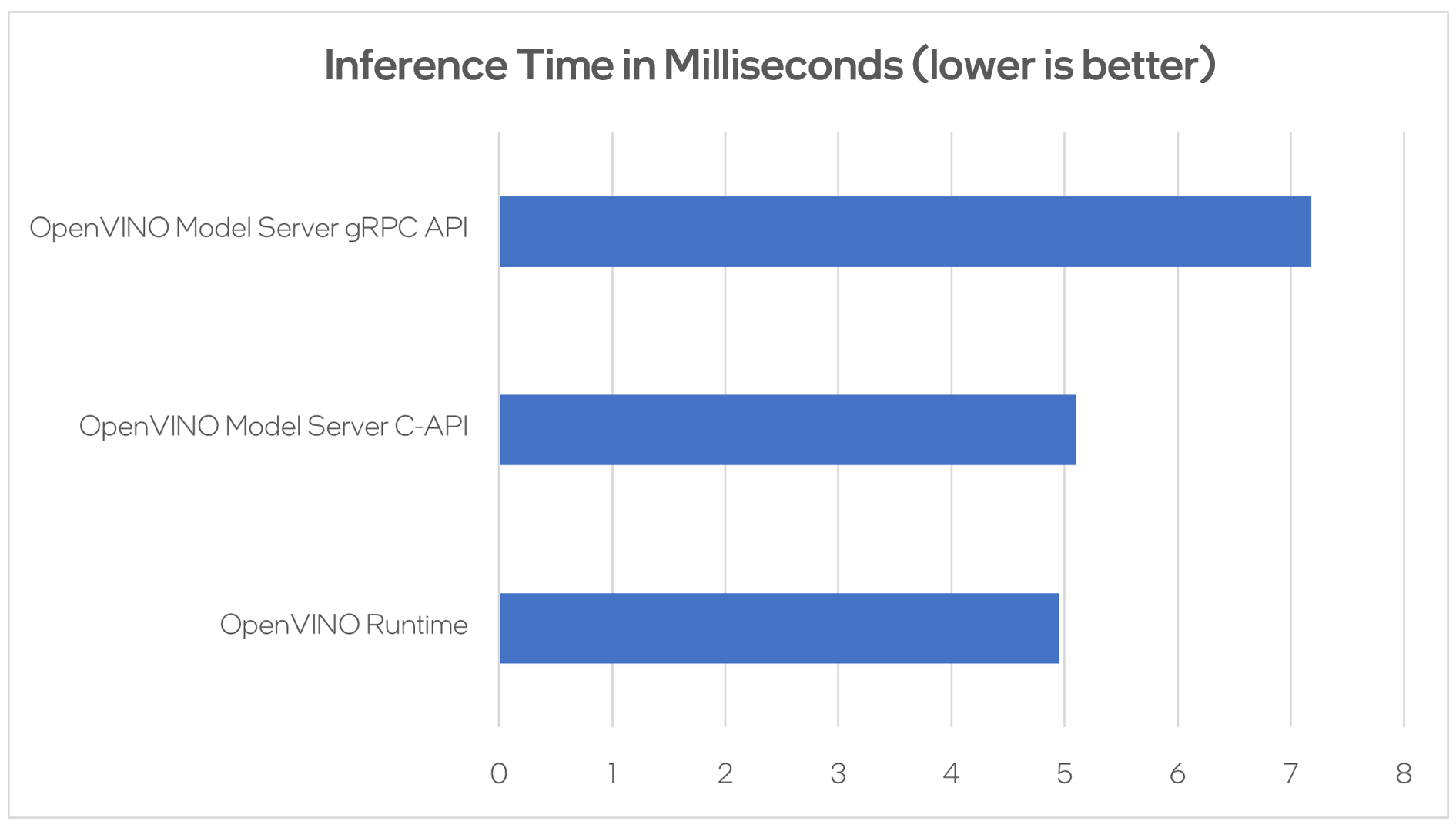
Using benchmarking tools from OpenVINO Runtime and both the C-API and gRPC API in OpenVINO Model Server, we can compare inference results via C-API to typical scenario of gRPC or direct integration of OpenVINO Runtime. The Resnet-50-tf model from Open Model Zoo was used for the testing below.

‍

Hardware configuration used:

- 1-node, Intel Xeon Gold 6252 @ 2.10GHz processor with 256GB (8 slots/16GB/2666) total DDR memory, HT on, Turbo on, Ubuntu 20.04.2 LTS,5.4.0-109-generic kernel

- Intel S2600WFT motherboard

Tested by Intel on 01/31/2023.

‍

Conclusion

With the new method of embedding OVMS into C++ applications, users can decrease inference latency even further by entirely skipping the networking part of model serving. The C-API is still in preview and has some limitations, but in its current state is ready to integrate into C++ applications. If you have questions or feedback, please file an issue on GitHub.

Read more:

• Complete API description: https://docs.openvino.ai/latest/ovms_docs_c_api.html  
• End to end demo: https://docs.openvino.ai/latest/ovms_demo_capi_inference_demo.html  

‍

Introduction

CPU plugin of OpenVINO™ toolkit as one of the most important part, which is powered by oneAPI Deep Neural Network Library (oneDNN) can help user achieve high performance inference of neural networks on Intel®x86-64 CPUs. The CPU plugin detects the Instruction Set Architecture (ISA) in the runtime and uses Just-in-Time (JIT) code generation to deploy the implementation optimized for the latest supported ISA.

In this blog, you will learn how layer primitives been optimized by implementation of ISA extensions and how to change the ISA extensions’ optimized kernel function at runtime for performance tuning and debugging.

After reading this blog, you will start to be proficient in AI workloads performance tuning and OpenVINO™ profiling on Intel® CPU architecture.

CPU Profiling

OpenVINO™ provide Application Program Interface (API) which is easy to turn on CPU profiling and analyze performance of each layer from the bottom level by executed kernel function. Firstly, enable performance counter profiling with executed device during device property configuration before model compiling with device. Learn detailed information from document of OpenVINO™ Configuring Devices.

core.set_property("CPU", ov::enable_profiling(true));

Then, you are allowed to get object of profiling info from inference requests which complied with the CPU device plugin.

auto perfCounts = infer_request.get_profiling_info();

Please note that performance profiling information generally can get after model inference. Refer below code implementation and add this part after model inference. You are possible to get status and performance of layer execution. Follow below code implement, you will get performance counter printing in order of the execution time from largest to smallest.

bool sort_pc_descend(const ov::ProfilingInfo& profiling1, const ov::ProfilingInfo& profiling2) {
    return profiling1.real_time > profiling2.real_time;
}
...
int tmain(int argc, tchar* argv[]) {
	...
	//objects init
	int layersize = 0;
	bool sort_pc_descend = 1;
	std::chrono::microseconds total = std::chrono::microseconds::zero();
	std::chrono::microseconds total_cpu = std::chrono::microseconds::zero();
	static const char* status_names[] = {"NOT_RUN", "OPTIMIZED_OUT", "EXECUTED"};

	//print row of title
	std::cout << "layerName\t"
	    << "execStatus\t"
	    << "layerType:"
	    << "execType\t";
	std::cout << "realTime (ms)\t"
	    << "cpuTime (ms)\t"
	    << " proportion(%)" << std::endl;

	//calculate executed layers total latency
	for (const auto& layer : perfCounts) {
	    if (std::string(status_names[(int)layer.status]).compare("EXECUTED") == 0) {
	        total += layer.real_time;
	        total_cpu += layer.cpu_time;
	    }
	}

	//print executed layer name, status, execution kernel funtion, CPU execution time and percentage of total model latency
	std::sort(perfCounts.begin(), perfCounts.end(), sort_pc_descend);
	for (const auto& layer : perfCounts) {
	    if (std::string(status_names[(int)layer.status]).compare("EXECUTED") == 0) {
	        std::cout << layer.node_name << "\t";
	        std::cout << ((int)layer.status < (sizeof(status_names) / sizeof(status_names[0]))
	                    ? status_names[(int)layer.status]
	                    : "INVALID_STATUS") << "\t";
	        std::cout << layer.node_type << ":" << layer.exec_type << "\t";
	        std::cout << std::to_string(layer.real_time.count() / 1000.0) << "\t"
	            << std::to_string(layer.cpu_time.count() / 1000.0) << "\t";
	        std::cout << (layer.real_time * 1.0 / total) * 100 << std::endl;
	        layersize += 1;
	    }
	}
}

CPU Dispatching

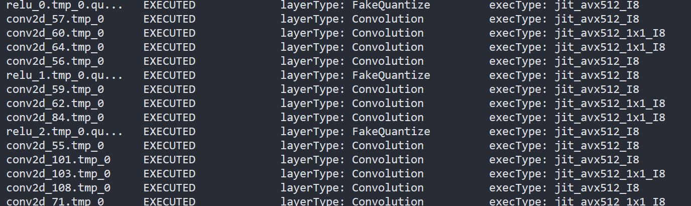
By enabling device profiling and printing exec_type of layers, you will get the specific kernel functions which powered by oneDNN during runtime execution. Use TensorFlow* ResNet 50 INT8 model for execution and pick the first 10 hotspot layers on 4th Gen Intel® Xeon Scalable processor (code named Sapphire Rapids) as an example:

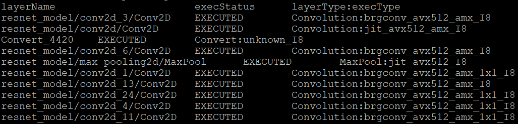
From execution type of layers, it would be helpful to check which oneDNN kernel function used, and the actual precision of layer execution and the optimization from supported ISA on this platform.

Normally, oneDNN is able to detect to certain ISA, and OpenVINO™ allow to use latest ISA with higher priority. If you want to compare optimization rate between different ISA, can use the ONEDNN_MAX_CPU_ISA environment variable to limit processor features with older instruction sets. Follow this link to check oneDNN supported ISA.

Please note, Intel® Advanced Matrix Extensions (Intel® AMX) ISA start to be supported since 4th Gen Intel® Xeon Scalable processor. You can refer Intel® Product Specifications to check the supported instruction set of your current platform.

The ISAs are partially ordered:

·      SSE41 < AVX < AVX2 < AVX2_VNNI <AVX2_VNNI_2,

·      AVX2 < AVX512_CORE < AVX512_CORE_VNNI< AVX512_CORE_BF16 < AVX512_CORE_FP16 < AVX512_CORE_AMX <AVX512_CORE_AMX_FP16,

·      AVX2_VNNI < AVX512_CORE_FP16.

To use CPU dispatcher control, just set the value of ONEDNN_MAX_CPU_ISA environment variable before executable program which contains the OpenVINO™ device profiling printing, you can use benchmark_app as an example:

ONEDNN_MAX_CPU_ISA=AVX512_CORE_VNNI benchmark_app -m ~/models/public/resnet-50-tf/FP32-INT8/resnet-50-tf.xml -d CPU -pcsort sort

The benchmark_app provides the option which named “-pcsort” can report performance counters and order analysis information by order of layers execution time when set value of the option by “sort”.

In this case, we use above code implementation can achieve similar functionality of benchmark_app “-pcsort” option. User can consider try to add the code implementation into your own OpenVINO™ program like below:

ONEDNN_MAX_CPU_ISA=AVX512_CORE_VNNI ./classification_profiling ~/models/public/resnet-50-tf/FP32-INT8/resnet-50-tf.xml ./sample_640×426.bmp CPU

After setting the CPU dispatcher, the kernel execution function has been switched from AVX512_CORE_AMX to AVX512_CORE_VNNI. Then, the performance counters information would be like below:

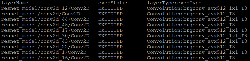
You can easily find the hotspot layers of the same model would be changed when executed by difference kernel function which optimized by implementation of different ISA extensions. That is also the optimization differences between architecture platforms.

Tuning Tips

Users can refer the CPU dispatcher control and OpenVINO™ device profiling API to realize performance tuning of your inference program between CPU architectures. It will also be helpful to developer finding out the place where has the potential space of performance improvement.

For example, the hotspot layer generally should be compute-intensive operations like matrix-matrix multiplication; General vector operations which is not target to artificial intelligence (AI) / machine learning (ML) workloads cannot be optimized by Intel® AMX and Intel® Deep Learning Boost (Intel® DL Boost), and the memory accessing operations, like Transpose which maybe cannot parallelly optimized with instruction sets. If your inference model remains large memory accessing operations rather than compute-intensive operations, you probably need to be focusing on RAM bandwidth optimization.

‍

OpenVINO empowers developers to write deep learning application code once and deploy it on a wide range of Intel hardware with best-in-class performance. Previously, significant effort had to be spent configuring inference pipelines to squeeze optimal performance out of target hardware, and the effort had to be repeated whenever the application was ported to a new platform. The new Auto Device Plugin (AUTO) and automatic configuration features in OpenVINO make it easier for developers to unlock performance on multiple hardware targets without needing to spend time optimizing their application pipeline.

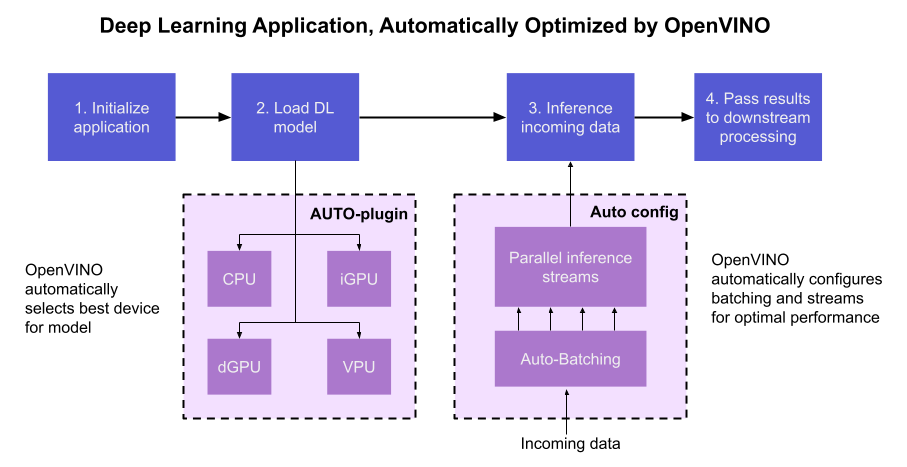
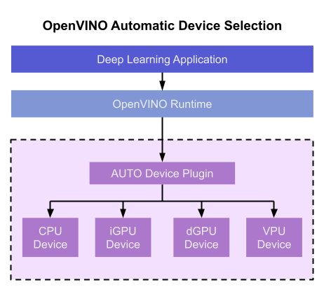
When an OpenVINO application is deployed in a system, the Auto Device Plugin automatically selects the best hardware target to inference the model with. OpenVINO then automatically configures the application to use optimal pipeline parameters based on the hardware capabilities and model size. Developers no longer need to write code for detecting hardware devices and explicitly configuring batch and stream parameters. High-level configuration is provided through performance hints that allow a developer to prioritize their application for either high throughput or minimal latency. AUTO and automatic device configuration make applications hardware-agnostic, allowing them to easily be ported to new hardware without any code changes.

The diagram in Figure 1 shows how OpenVINO’s features automatically configure an application for optimal performance, regardless of the target hardware. When the deep learning model is loaded, AUTO creates a transparent plugin interface to the available processor devices and automatically selects the most suitable device. OpenVINO configures the batch size and number of processing streams based on the selected hardware target, and the Auto-Batching feature automatically groups incoming data into optimally sized batches. AUTO and automatic configuration operate independently from each other, so developers can use either or both in their application.

AUTO and automatic configuration are available starting in the 2022.1 release of OpenVINO Runtime. To use these features, simply install OpenVINO Runtime on the target hardware. The API uses AUTO by default if no processor device is specified when loading a model. Set a “throughput” or “latency” performance hint when loading the model, and the API automatically configures the inference pipeline. Read on to learn more about AUTO, automatic configuration, performance hints, and how to use them in your application.

‍

Automatic Device Selection

Auto Device Plugin (AUTO) is a “virtual” device that provides a transparent interface to physical devices in the system. When an application is initialized, AUTO discovers the available processors and accelerators in the system (CPUs, integrated GPUs, discrete GPUs, VPUs) and selects the best device, based on a default device priority list or an optional user-provided priority list. It creates an interface between the application and device that executes inference requests in an optimized fashion. It enables an application to always achieve optimal performance in a system without the developer having to know beforehand what devices are available in the system.

Key Features and Benefits

Simple and flexible application deployment

Previously, developers needed to know details about target hardware and configure their application specifically for each device. AUTO removes the need to write dedicated code for specific devices. This enables an application to be written once and deployed to any supported hardware. It also allows the application to run on newer generations of hardware as they are released: the developer only needs to compile the application with the latest version of OpenVINO to run it on new hardware. This provides an instant increase in performance with little development time.

‍

Configurability

AUTO provides a configuration interface that is easy to use at a high level while still providing flexibility. Developers can simply specify “AUTO” as the device to tell the application to select the best device for the given model. They can also control which device is selected by providing a device candidate list and setting priorities for each device. 

Developers can also use performance hints to configure their application for latency or throughput. When the performance hint is throughput, OpenVINO will create more streams for parallel inferencing to achieve maximum processing bandwidth. In latency mode, OpenVINO creates fewer streams to utilize as many resources as possible to complete each inference quickly. Performance hints also help determine the optimal batch size for inferencing; this is discussed further in the “Performance Hints” section of this document.

‍

Improved first-inference latency

In applications that use accelerated processors like GPUs or VPUs, the time to first inference may be higher than average because it takes time to compile and load the deep learning model into the accelerator. AUTO solves this problem by starting the first inference with the CPU, which has minimal latency and no delays. As the first inference is being performed, AUTO continues to compile and load the model for the selected accelerator device, and then transparently switches over to that device when it is ready. This significantly reduces time to first inference, and is beneficial for applications that require immediate inference results on startup.

‍

How Automatic Device Selection Works

To choose the best device for inference, AUTO discovers which hardware targets are available in the system and matches the model to the best supported device, using the following process:

‍

1. AUTO discovers which devices are available using the Query Device API. The query reads an internal file that lists installed hardware plugins, confirms the hardware modules are present by communicating with them through drivers, and returns a list of available devices in the system.
   
   
2. AUTO checks the precision of the input model by reading the model file.
   
   
3. AUTO selects the best available device in the device priority table (shown in Table 1 below) that is capable of supporting the model’s precision.
   
   
4. AUTO attempts to compile the model on the selected device. If the model doesn’t compile (for example, if the device doesn’t support all the operations required by the model), AUTO tries to compile it on the next best device until compilation is successful. The CPU is the final fallback device, as it supports all operations and precisions.

‍

By default, AUTO uses the device priority list shown in Table 1. Developers can customize the table to provide their own device priority list and limit the devices that are available to run inferencing. AUTO will not try to run inference on devices that are not provided in the device list.

‍

Table 1. Default AUTO Device Priority List

‍

As mentioned, AUTO reduces the first inference latency by compiling and loading the model to the CPU first. As the model is loaded to the CPU and first inference is performed, AUTO steps through the rest of the process for selecting the device and compiling the model to that device. This way, devices that require a long time for model compilation do not impede inference as the application is being initialized.

AUTO also provides a model priority feature that enables developers to control which models are loaded to which devices when there are multiple models running on a system with multiple devices. Developers can set “MODEL_PRIORITY” as “HIGH”, “MEDIUM”, or “LOW” to configure which models should be allocated to the best resource. This allows developers to ensure models that are critical for an application are always loaded to the fastest device for processing, while less critical models are loaded to slower devices.

For example, consider a medical imaging application with models for segmenting and/or classifying injuries in X-ray images running on a system that has both a GPU and a CPU. The segmentation model is set to HIGH priority because it takes more processing power to inference, while the classification model is set to MEDIUM priority. If both models are loaded at the same time, the segmentation model will be loaded to the GPU (the higher priority device) and the classification model will be loaded to the CPU (the lower priority device). If only the classification model is loaded, it will be loaded to the GPU since the GPU isn’t occupied by the higher-priority model.

Automatic Device Configuration

The performance of a deep learning application can be improved by configuring runtime parameters to fully utilize the target hardware. There are several factors to take into consideration when optimizing inference for a certain device, such as batch size and number of streams. (See Runtime Inference Optimizations in OpenVINO documentation for more information.) The optimal configuration for these parameters depends on the architecture and memory of the target hardware, and they need to be re-determined when porting an application from one device to another. 

OpenVINO provides features that automatically configure an application to use optimal runtime parameters to achieve the best performance on any supported hardware target. These features are enabled through performance hints, which allow a user to specify whether their application should be optimized for latency or throughput. The automatic configuration eliminates the time and effort required to determine optimal configurations. It makes it simple to port to new devices or write one application to work on multiple devices. OpenVINO’s automatic configuration features currently work with CPU and GPU devices, and support for VPUs will be added in a future release.

‍

Performance Hints

OpenVINO allows users to provide high-level "performance hints" for setting latency-focused or throughput-focused inference modes. These performance hints are “latency” and “throughput.” The hints cause the runtime to automatically adjust runtime parameters, such as number of processing streams and inference batch size, to prioritize for reduced latency or high throughput. Performance hints are supported by CPU and GPU devices, and a future release of OpenVINO will add support for VPUs.

The performance hints do not require any device-specific settings and are portable between devices. Parameters are automatically configured based on whichever device is being used. This allows users to easily port applications between hardware targets without having to re-determine the best runtime parameters for the new device.

Latency performance hint

Latency is the amount of time it takes to process a single inference request and is usually measured in milliseconds (ms). In applications where data needs to be inferenced and acted on as quickly as possible (such as autonomous driving), low latency is desirable. When applications are run with the “latency” performance hint, OpenVINO determines the optimal number of parallel inference requests for minimizing latency while still maximizing the parallelization capabilities of the hardware. It automatically sets the number of processing streams to achieve the best latency.

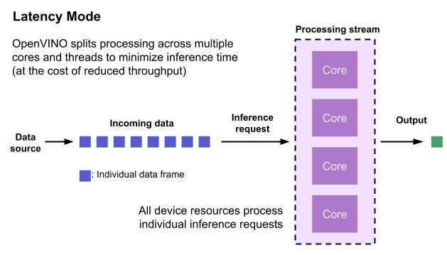
To achieve the fastest latency, the processor device should process only one inference request at a time so all the compute resources are available for calculation. However, devices with multiple cores (such as multi-socket CPUs or multi-tile GPUs) can deliver multiple streams with the same latency as they would with a single stream. OpenVINO automatically checks the compute demands of the model, queries capabilities of the device, and selects the number of streams to be the minimum required to get the best latency. For CPUs, this is typically one stream for each socket. For GPUs, it’s typically one stream per tile.

Throughput performance hint

Throughput is the amount of data an inferencing pipeline can process at once, and it is usually measured in frames per second (FPS) or inferences per second. In applications where large amounts of data needs to be inferenced simultaneously (such as multi-camera video streams), high throughput is needed. To achieve high throughput, the runtime should focus on fully saturating the device with enough data to process. When applications are run with the “throughput” performance hint, OpenVINO maximizes the number of parallel inference requests to utilize all the threads available on the device. On GPU, it automatically sets the inference batch size to fill up the GPU memory available.

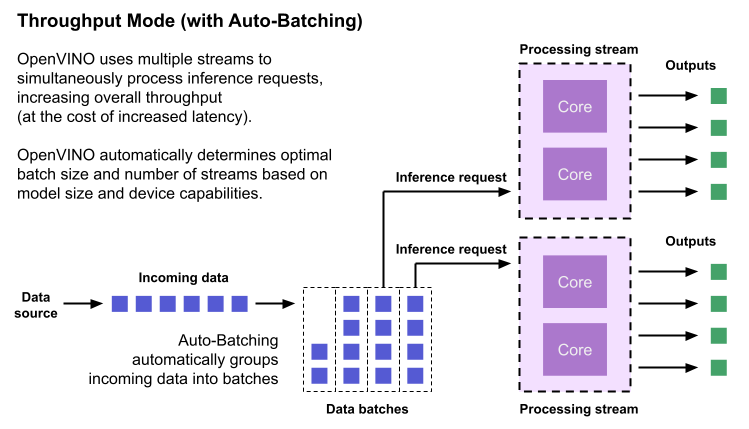
To configure the runtime for high throughput, OpenVINO automatically sets the number of streams to use based on the architecture of the device. For CPUs, it creates as many streams as there are cores available. For GPUs, it uses a combination of batch size and parallel streams to fully utilize the GPU’s memory and compute resources. To determine the optimal configuration on GPUs, OpenVINO will first check if the network supports batching. If it does, it loads the network with a batch size of one, determines how much memory is used for the single-batch network, and then scales the batch size and streams up to fill the entire GPU.

Batch size can also be explicitly specified in code when the model is loaded. This can be useful in applications where the number of incoming data sources is known and constant. For example, in an application that processes four camera streams, specify a batch size of four so that each set of frames from the cameras is processed in a single inference request. More information on batch configuration is given in the Auto-Batching section below.

‍

Auto-Batching

Auto-Batching is a new feature of OpenVINO that performs on-the-fly grouping of data inference requests in an application. As the application makes individual inference requests, Auto-Batching transparently collects them into a batch. When the batch is full (or when a timeout limit is reached), OpenVINO executes inference on the whole batch. In short, it takes care of batching data efficiently so the developer doesn’t have to worry about it.

The Auto-Batching feature is controlled by the configuration parameter “ALLOW_AUTO_BATCHING”, which is enabled by default. Auto-Batching is activated when all of the following are true:

• ALLOW_AUTO_BATCHING is true
• The model is loaded to the target device with the throughput performance hint
• The target device supports batching (such as GPU)
• The model topology supports batching

‍

When Auto-Batching is activated, OpenVINO automatically determines the optimal batch size for an application based on model size and hardware capabilities. Developers can also explicitly specify the batch size when loading the model. While the inference pipeline is active, individual inference requests are gathered into a batch and then executed when the batch is full.

Auto-Batching also has a timeout feature that is configurable by the developer. If there aren’t enough individual requests collected within the developer-specified time limit, batch execution will fall back to just using individual inference requests. For example, a developer may specify a timeout limit of 500 ms and a batch size of 16 for a video processing inference pipeline. Once 16 frames are gathered, a batch inference request is made. If only 13 frames arrive before the 500 ms timeout is hit, the application will perform individual inference requests on each of the 13 frames. While the timeout feature makes the pipeline robust to interruptions in incoming data, hitting the timeout limit heavily reduces the performance. To avoid this, developers should make sure there is enough incoming data to fill the batch within the time limit in typical conditions.

Auto-Batching, when combined with OpenVINO's automatic configuration features that determine optimal batch size and number of streams, provides a powerful benefit to the developer. The developer can utilize the full power of the target device with only using one line of code. Best of all, when an application is used on a different device, it will automatically reconfigure itself to achieve optimal performance with zero effort from the developer.

How to Use AUTO and Performance Hints

Using AUTO and automatic configuration with performance hints only requires one line of code. The functionality centers around the “ie.compile_model” method, which is used to compile a model and load it into device memory. The method accepts various configuration parameters that allow a user to provide high-level control over the pipeline.

Here are several Python examples showing how to configure a model and pipeline with the ie.compile_model method. The first example also shows how to import the OpenVINO Core model, initialize it, and read a model before calling ie.compile_model.

‍

Example 1. Load a model on AUTO device

from openvino.runtime import Core

ie = Core() # Initialize inference engine
model = ie.read_model(model="model.xml") # Read the model file

# Load model onto AUTO device
compiled_model = ie.compile_model(model=model, device_name="AUTO")

‍

Example 2. Load a model on AUTO device with performance hints

# Load model using the THROUGHPUT performance hint
compiled_model = core.compile_model(model=model, device_name="AUTO", config={"PERFORMANCE_HINT":"THROUGHPUT"}

# Alternatively, load model using the LATENCY performance hint
compiled_model = core.compile_model(model=model, device_name="AUTO", config={"PERFORMANCE_HINT":"LATENCY"})

‍

Example 3. Provide a list of device candidates which AUTO may use when loading a model

# Specify that AUTO can use either the GPU or CPU device
compiled_model = core.compile_model(model=model, device_name="AUTO:GPU,CPU")

‍

‍Example 4. Load multiple models with HIGH, MEDIUM, and LOW priorities

# Load three models and set them as HIGH, MEDIUM, and LOW priority
compiled_model0 = core.compile_model(model=model, device_name="AUTO", config={"MODEL_PRIORITY":"HIGH"})

compiled_model1 = core.compile_model(model=model, device_name="AUTO", config={"MODEL_PRIORITY":"MEDIUM"})

compiled_model2 = core.compile_model(model=model, device_name="AUTO", config={"MODEL_PRIORITY":"LOW"})

‍

‍Example 5. Load a model to GPU and use Auto-Batching with an explicitly set batch size

# Load model to GPU in throughput mode, with batch size set to 4
# (i.e. Auto-Batching collects 4 individual batches and then runs them all at once)
compiled_model = core.compile_model(model, "BATCH:GPU(4)", {"PERFORMANCE_HINT": "THROUGHPUT"})

‍

For a more in-depth example of how to use AUTO and automatic configuration, please visit the Automatic Device Selection with OpenVINO Jupyter notebook in the OpenVINO notebooks repository. It provides an end-to-end example that shows:

1. How to download a model from Open Model Zoo and convert it to OpenVINO IR format with Model Optimizer
2. How to load a model to AUTO device
3. The improvement in first inference latency when using AUTO device
4. How to perform asynchronous inferencing on data batches in throughput or latency mode
5. A performance comparison between throughput and latency modes

The OpenVINO Benchmark App also serves as a useful tool for experimenting with devices and batching to see how performance changes under various configurations. The Benchmark App supports automatic device selection and performance hints for throughput or latency.

Where to Learn More

To learn more please visit auto device plugin and automatic configuration pages in OpenVINO documentation. They provide more information about how to use and configure them in an application.

OpenVINO also provides an example notebook explaining how to use AUTO and showing how it improves performance. The notebook can be downloaded and run on a development machine where OpenVINO Developer Tools have been installed. Visit the notebook at this link: Automatic Device Selection with OpenVINO.

To learn more about OpenVINO toolkit and how to use it to build optimized deep learning applications, visit the Get Started page. OpenVINO also provides a number of example notebooks showing how to use it for basic applications like object detection and speech recognition on the Tutorials page.

Authors: Alexander Kozlov, Vui Seng Chua, Yujie Pan, Rajesh Poornachandran, Sreekanth Yalachigere, Dmitry Gorokhov, Nilesh Jain, Ravi Iyer, Yury Gorbachev

Introduction

When it comes to the inference of overparametrized Deep Neural Networks, perhaps, weight pruning is one of the most popular and promising techniques that is used to reduce model footprint, decrease the memory throughput required for inference, and finally improve performance. Since Language Models (LMs) are highly overparametrized and contain lots of MatMul operations with weights it looks natural to prune the redundant weights and benefit from sparsity at inference time. There are several types of pruning methods available:

• Fine-grained pruning (single weights).
• Coarse pruning: group-level pruning (groups of weights), vector pruning (rows in weights matrices), and filter pruning (filters in ConvNets).

Contemporary Language Models are basically represented by Transformer-based architectures. Using coarse pruning methods for such models is problematic because of the many connections between the layers. This trait means that, first, not every pruning type is applicable to such models and, second, pruning of some dimension in one layer requires adjustments in the rest of the layers connected to it.

Fine-grained sparsity does not have such a constraint and can be applied to each layer independently. However, it requires special support on the HW and inference SW level to get real performance improvements from weight sparsity. There are two main approaches that help to leverage from weight sparsity at inference:

• Skip multiplication and addition for zero weights in dot products of weights and activations. This usually results in a special instruction set that implements such logic.
• Weights compression/decompression to reduce the memory throughput. Compression is performed at the model load/compilation stage while decompression happens on the fly right before the computation when weights are in the cache. Such a method can be implemented on the HW or SW level.

In this blog post, we focus on the SW weight decompression method and showcase the end-to-end workflow from model optimization to deployment with OpenVINO.

Sparsity support in OpenVINO

Starting from OpenVINO 2022.3release, OpenVINO runtime contains a feature that enables weights compression/decompression that can lead to performance improvement on the 4thGen Intel® Xeon® Scalable Processors. However, there are some prerequisites that should be considered to enable this feature during the model deployment:

• Currently, this feature is available only to MatMul operations with weights (Fully-connected layers). So currently, there is no support for sparse Convolutional layers or other operations.
• MatMul layers should contain a high level of weights sparsity, for example, 80% or higher which is achievable, especially for large Transformer models trained on simple tasks such as Text Classification.
• The deployment scenario should be memory-bound. For example, this prerequisite is applicable to cloud deployment when there are multiple containers running inference of the same model in parallel and competing for the same RAM and CPU resources.

The first two prerequisites assume that the model is pruned using special optimization methods designed to introduce sparsity in weight matrices. It is worth noting that pruning methods require model fine-tuning on the target dataset in order to reduce accuracy degradation caused by zeroing out weights within the model. It assumes the availability of the HW capable of DL model training. Nowadays, many frameworks and libraries offer such methods. For example, PyTorch provides some capabilities for NN pruning. There are also resources that offer pre-trained sparse models that can be used as a starting point, for example, SparseZoo from Neural Magic.

OpenVINO also provides instruments for DL model pruning implemented in Neural Network Compression Framework (NNCF) that is aimed specifically for model optimization and offers different optimization options: from post-training optimization to deep compression when stacking several optimization methods. NNCF is also integrated into Hugging Face Optimum library which is designed to optimize NLP models from Hugging Face Hub.

Using only sparsity is not so beneficial compared to another popular optimization method such as bit quantization which can guarantee better performance-accuracy trade-offs after optimization in the general case. However, the good thing about sparsity is that it can be stacked with 8-bit quantization so that the performance improvements of one method reinforce the optimization effect of another one leading to a higher cumulative speedup when applying both. Considering this, OpenVINO runtime provides an acceleration feature for sparse and 8-bit quantized models. The runtime flow is shown in the scheme below:

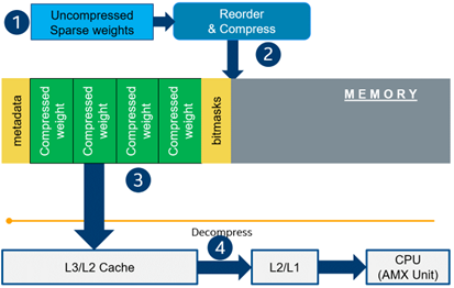
Below, we demonstrate two end-to-end workflows:

• ‍Pruning and 8-bit quantization of the floating-point BERT model using Hugging Face Optimum and NNCF as an optimization backend.
• ‍Quantization of sparse BERT model pruned with 3^rd party optimization solution.

Both workflows end up with inference using OpenVINO API where we show how to turn on a runtime option that allows leveraging from sparse weights.

Pruning and 8-bit quantization with Hugging Face Optimum and NNCF

This flow assumes that there is a Transformer model coming from the Hugging Face Transformers library that is fine-tuned for a downstream task. In this example, we will consider the text classification problem, in particular the SST2 dataset from the GLUE benchmark, and the BERT-base model fine-tuned for it. To do the optimization, we used an Optimum-Intel library which contains the optimization capabilities based on the NNCF framework and is designed for inference with OpenVINO. You can find the exact characteristics and steps to reproduce the result in this model card on the Hugging Face Hub. The model is 80% sparse and 8-bit quantized.

To run a pre-optimized model you can use the following code from this notebook:

from pathlib import Path

from optimum.intel.openvino import OVModelForSequenceClassification
from transformers import AutoTokenizer, pipeline
from huggingface_hub import hf_hub_download

model_id = "OpenVINO/bert-base-uncased-sst2-int8-unstructured80"
ov_model = OVModelForSequenceClassification.from_pretrained(model_id)
tokenizer = AutoTokenizer.from_pretrained(model_id)

Quantization of already pruned model

In case if you deal with already pruned model, you can use Post-Training Quantization from the Optimum-Intel library to make it 8-bit quantized as well. The code snippet below shows how to quantize the sparse BERT model optimized for MNLI dataset using Neural Magic SW solution. This model is publicly available so that we download it using Optimum API and quantize on fly using calibration data from MNLI dataset. The code snippet below shows how to do that.

from functools import partial
from pathlib import Path

from datasets import load_dataset
from transformers import AutoModelForSequenceClassification, AutoTokenizer

from optimum.intel.openvino import OVQuantizer
from optimum.intel.openvino import OVConfig

model_id = "neuralmagic/oBERT-12-downstream-pruned-unstructured-90-mnli"
quantized_sparse_dir = Path("bert_90_sparse_quantized")

# Instantiate model and tokenizer in PyTorch and load them from the HF Hub
torch_model = AutoModelForSequenceClassification.from_pretrained(model_id)
tokenizer = AutoTokenizer.from_pretrained(model_id)

def preprocess_function(examples, tokenizer):
    """
    Define a function that tokenizes the data and returns it in the format expected by the model.
    
    :param: examples: a dictionary containing the input data which are the items from caliration dataset.
            tokenizer: a tokenizer object that is used to tokenize the text data.
    :returns:
            the data that can be fed directly to the model.
    """
    return tokenizer(
        examples["premise"], examples["hypothesis"], padding="max_length", max_length=128, truncation=True
    )

# Create quantization config (default) and OVQuantizer
# OVConfig is a wrapper class on top of NNCF config. 
# Use "compression" field to control quantization parameters
# For more information about the parameters refer to NNCF GitHub documentatioin
quantization_config = OVConfig()
quantizer = OVQuantizer.from_pretrained(torch_model, feature="sequence-classification")

# Instantiate a dataset and convert it to calibration dataset using HF API
# The latter one produces a model input
dataset = load_dataset("glue", "mnli")
calibration_dataset = quantizer.get_calibration_dataset(
    "glue",
    dataset_config_name="mnli",
    preprocess_function=partial(preprocess_function, tokenizer=tokenizer),
    num_samples=100,
    dataset_split="train",
)
# Apply static quantization and export the resulting quantized model to OpenVINO IR format
quantizer.quantize(
    quantization_config=quantization_config, calibration_dataset=calibration_dataset, save_directory=quantized_sparse_dir
)

Enabling sparsity optimization inOpenVINO Runtime and 4th Gen Intel® Xeon® Scalable Processors

Once you get ready with the sparse quantized model you can use the latest advances of the OpenVINO runtime to speed up such models. The model compression feature is enabled in the runtime at the model compilation step using a special option called: “CPU_SPARSE_WEIGHTS_DECOMPRESSION_RATE”. Its value controls the minimum sparsity rate that MatMul operation should have to be optimized at inference time. This property is passed to the compile_model API as it is shown below:

from openvino.runtime import Core

core = Core()
model = core.read_model(model="path_to_model_xml")
# MatMul layers with higher sparsity rate than 80% are optimized
configuration = {"CPU_SPARSE_WEIGHTS_DECOMPRESSION_RATE": 0.8} 
compiled_model = core.compile_model(model=model, device_name="CPU", config=configuration)

An important note is that a high sparsity rate is required to see the performance benefit from this feature. And we note again that this feature is available only on the 4th Gen Intel® Xeon® Scalable Processors and it is basically for throughput-oriented scenarios. To simulate such a scenario, you can use the benchmark_app application supplied with OpenVINO distribution and limit the number of resources available for inference. Below we show the performance difference between the two runs sparsity optimization in the runtime:

• Benchmarking without sparsity optimization:

# Dump benchmarking config for dense inference
with open("perf_config.json", "w") as outfile:
    outfile.write(
        """
        {
            "CPU": {"NUM_STREAMS": 4, "INFERENCE_NUM_THREADS": 4}
        }
        """
    )
benchmark_app -m bert_90_sparse_quantized/openvino_model.xml -shape "input_ids[1,16],attention_mask[1,16],token_type_ids[1,16]" -load_config perf_config.json

• Benchmarking when sparsity optimization is enabled:

# Dump benchmarking config for sparse inference
with open("perf_config_sparse.json", "w") as outfile:
    outfile.write(
        """
        {
            "CPU": {"NUM_STREAMS": 4, "INFERENCE_NUM_THREADS": 4, "CPU_SPARSE_WEIGHTS_DECOMPRESSION_RATE": 0.8}
        }
        """
    )
benchmark_app -m bert_90_sparse_quantized/openvino_model.xml -shape "input_ids[1,16],attention_mask[1,16],token_type_ids[1,16]" -load_config perf_config_sparse.json

Performance Results

We performed a benchmarking of our sparse and 8-bit quantized BERT model on 4th Gen Intel® Xeon® Scalable Processors with various settings. We ran two series of experiments where we vary the number of parallel threads and streams available for the asynchronous inference in the first experiments and we investigate how the sequence length impact the relative speedup in the second series of experiments.

The table below shows relative speedup for various combinations of number of streams and threads and at the fixed sequence length after enabling sparsity acceleration in the OpenVINO runtime.

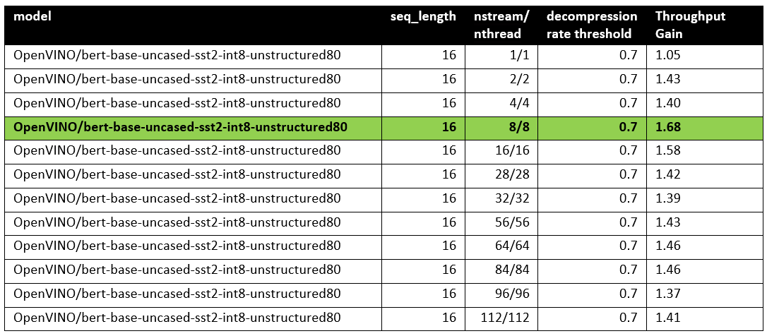
Based on this, we can conclude that one can expect significant performance improvement with any number of streams/threads larger than one. The optimal performance is achieved at eight streams/threads. However, we would like to note that this is model specific and depends on the model architecture and sparsity distribution.

The chart below also shows the relationship between the possible acceleration and the sequence length.

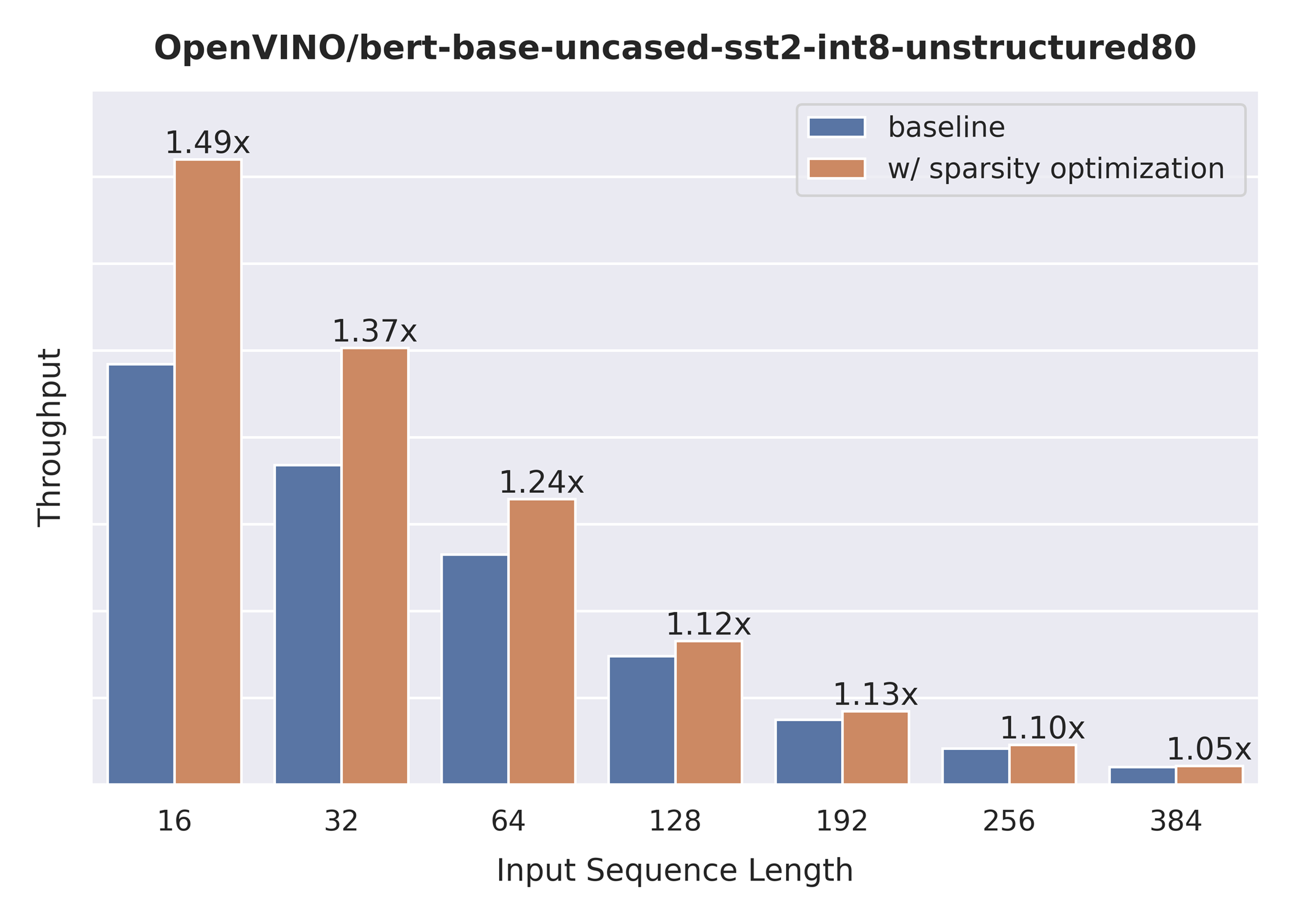
As you can see the benefit from sparsity is decreasing with the growth of the sequence length processed by the model. This effect can be explained by the fact that for larger sequence lengths the size of the weights is no longer a performance bottleneck and weight compression does not have so much impact on the inference time. It means that such a weight sparsity acceleration feature does not suit well for large text processing tasks but could be very helpful for Question Answering, Sequence Classification, and similar tasks.

^References

• Jupyter notebook with the performance benchmarks.
• Model card for sparse and quantized BERT-base model