Authors: Alexander Kozlov, Vui Seng Chua, Yujie Pan, Rajesh Poornachandran, Sreekanth Yalachigere, Dmitry Gorokhov, Nilesh Jain, Ravi Iyer, Yury Gorbachev
Introduction
When it comes to the inference of overparametrized Deep Neural Networks, perhaps, weight pruning is one of the most popular and promising techniques that is used to reduce model footprint, decrease the memory throughput required for inference, and finally improve performance. Since Language Models (LMs) are highly overparametrized and contain lots of MatMul operations with weights it looks natural to prune the redundant weights and benefit from sparsity at inference time. There are several types of pruning methods available:
Fine-grained pruning (single weights).
Coarse pruning: group-level pruning (groups of weights), vector pruning (rows in weights matrices), and filter pruning (filters in ConvNets).
Contemporary Language Models are basically represented by Transformer-based architectures. Using coarse pruning methods for such models is problematic because of the many connections between the layers. This trait means that, first, not every pruning type is applicable to such models and, second, pruning of some dimension in one layer requires adjustments in the rest of the layers connected to it.
Fine-grained sparsity does not have such a constraint and can be applied to each layer independently. However, it requires special support on the HW and inference SW level to get real performance improvements from weight sparsity. There are two main approaches that help to leverage from weight sparsity at inference:
Skip multiplication and addition for zero weights in dot products of weights and activations. This usually results in a special instruction set that implements such logic.
Weights compression/decompression to reduce the memory throughput. Compression is performed at the model load/compilation stage while decompression happens on the fly right before the computation when weights are in the cache. Such a method can be implemented on the HW or SW level.
In this blog post, we focus on the SW weight decompression method and showcase the end-to-end workflow from model optimization to deployment with OpenVINO.
Sparsity support in OpenVINO
Starting from OpenVINO 2022.3release, OpenVINO runtime contains a feature that enables weights compression/decompression that can lead to performance improvement on the 4thGen Intel® Xeon® Scalable Processors. However, there are some prerequisites that should be considered to enable this feature during the model deployment:
Currently, this feature is available only to MatMul operations with weights (Fully-connected layers). So currently, there is no support for sparse Convolutional layers or other operations.
MatMul layers should contain a high level of weights sparsity, for example, 80% or higher which is achievable, especially for large Transformer models trained on simple tasks such as Text Classification.
The deployment scenario should be memory-bound. For example, this prerequisite is applicable to cloud deployment when there are multiple containers running inference of the same model in parallel and competing for the same RAM and CPU resources.
The first two prerequisites assume that the model is pruned using special optimization methods designed to introduce sparsity in weight matrices. It is worth noting that pruning methods require model fine-tuning on the target dataset in order to reduce accuracy degradation caused by zeroing out weights within the model. It assumes the availability of the HW capable of DL model training. Nowadays, many frameworks and libraries offer such methods. For example, PyTorch provides some capabilities for NN pruning. There are also resources that offer pre-trained sparse models that can be used as a starting point, for example, SparseZoo from Neural Magic.
OpenVINO also provides instruments for DL model pruning implemented in Neural Network Compression Framework (NNCF) that is aimed specifically for model optimization and offers different optimization options: from post-training optimization to deep compression when stacking several optimization methods. NNCF is also integrated into Hugging Face Optimum library which is designed to optimize NLP models from Hugging Face Hub.
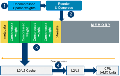
Using only sparsity is not so beneficial compared to another popular optimization method such as bit quantization which can guarantee better performance-accuracy trade-offs after optimization in the general case. However, the good thing about sparsity is that it can be stacked with 8-bit quantization so that the performance improvements of one method reinforce the optimization effect of another one leading to a higher cumulative speedup when applying both. Considering this, OpenVINO runtime provides an acceleration feature for sparse and 8-bit quantized models. The runtime flow is shown in the scheme below:
Below, we demonstrate two end-to-end workflows:
Pruning and 8-bit quantization of the floating-point BERT model using Hugging Face Optimum and NNCF as an optimization backend.
Quantization of sparse BERT model pruned with 3rd party optimization solution.
Both workflows end up with inference using OpenVINO API where we show how to turn on a runtime option that allows leveraging from sparse weights.
Pruning and 8-bit quantization with Hugging Face Optimum and NNCF
This flow assumes that there is a Transformer model coming from the Hugging Face Transformers library that is fine-tuned for a downstream task. In this example, we will consider the text classification problem, in particular the SST2 dataset from the GLUE benchmark, and the BERT-base model fine-tuned for it. To do the optimization, we used an Optimum-Intel library which contains the optimization capabilities based on the NNCF framework and is designed for inference with OpenVINO. You can find the exact characteristics and steps to reproduce the result in this model card on the Hugging Face Hub. The model is 80% sparse and 8-bit quantized.
To run a pre-optimized model you can use the following code from this notebook:
from pathlib import Path
from optimum.intel.openvino import OVModelForSequenceClassification
from transformers import AutoTokenizer, pipeline
from huggingface_hub import hf_hub_download
model_id = "OpenVINO/bert-base-uncased-sst2-int8-unstructured80"
ov_model = OVModelForSequenceClassification.from_pretrained(model_id)
tokenizer = AutoTokenizer.from_pretrained(model_id)
Quantization of already pruned model
In case if you deal with already pruned model, you can use Post-Training Quantization from the Optimum-Intel library to make it 8-bit quantized as well. The code snippet below shows how to quantize the sparse BERT model optimized for MNLI dataset using Neural Magic SW solution. This model is publicly available so that we download it using Optimum API and quantize on fly using calibration data from MNLI dataset. The code snippet below shows how to do that.
from functools import partial
from pathlib import Path
from datasets import load_dataset
from transformers import AutoModelForSequenceClassification, AutoTokenizer
from optimum.intel.openvino import OVQuantizer
from optimum.intel.openvino import OVConfig
model_id = "neuralmagic/oBERT-12-downstream-pruned-unstructured-90-mnli"
quantized_sparse_dir = Path("bert_90_sparse_quantized")
# Instantiate model and tokenizer in PyTorch and load them from the HF Hub
torch_model = AutoModelForSequenceClassification.from_pretrained(model_id)
tokenizer = AutoTokenizer.from_pretrained(model_id)
def preprocess_function(examples, tokenizer):
"""
Define a function that tokenizes the data and returns it in the format expected by the model.
:param: examples: a dictionary containing the input data which are the items from caliration dataset.
tokenizer: a tokenizer object that is used to tokenize the text data.
:returns:
the data that can be fed directly to the model.
"""
return tokenizer(
examples["premise"], examples["hypothesis"], padding="max_length", max_length=128, truncation=True
)
# Create quantization config (default) and OVQuantizer
# OVConfig is a wrapper class on top of NNCF config.
# Use "compression" field to control quantization parameters
# For more information about the parameters refer to NNCF GitHub documentatioin
quantization_config = OVConfig()
quantizer = OVQuantizer.from_pretrained(torch_model, feature="sequence-classification")
# Instantiate a dataset and convert it to calibration dataset using HF API
# The latter one produces a model input
dataset = load_dataset("glue", "mnli")
calibration_dataset = quantizer.get_calibration_dataset(
"glue",
dataset_config_name="mnli",
preprocess_function=partial(preprocess_function, tokenizer=tokenizer),
num_samples=100,
dataset_split="train",
)
# Apply static quantization and export the resulting quantized model to OpenVINO IR format
quantizer.quantize(
quantization_config=quantization_config, calibration_dataset=calibration_dataset, save_directory=quantized_sparse_dir
)
Enabling sparsity optimization inOpenVINO Runtime and 4th Gen Intel® Xeon® Scalable Processors
Once you get ready with the sparse quantized model you can use the latest advances of the OpenVINO runtime to speed up such models. The model compression feature is enabled in the runtime at the model compilation step using a special option called: “CPU_SPARSE_WEIGHTS_DECOMPRESSION_RATE”. Its value controls the minimum sparsity rate that MatMul operation should have to be optimized at inference time. This property is passed to the compile_model API as it is shown below:
from openvino.runtime import Core
core = Core()
model = core.read_model(model="path_to_model_xml")
# MatMul layers with higher sparsity rate than 80% are optimized
configuration = {"CPU_SPARSE_WEIGHTS_DECOMPRESSION_RATE": 0.8}
compiled_model = core.compile_model(model=model, device_name="CPU", config=configuration)
An important note is that a high sparsity rate is required to see the performance benefit from this feature. And we note again that this feature is available only on the 4th Gen Intel® Xeon® Scalable Processors and it is basically for throughput-oriented scenarios. To simulate such a scenario, you can use the benchmark_app application supplied with OpenVINO distribution and limit the number of resources available for inference. Below we show the performance difference between the two runs sparsity optimization in the runtime:
Benchmarking without sparsity optimization:
# Dump benchmarking config for dense inference
with open("perf_config.json", "w") as outfile:
outfile.write(
"""
{
"CPU": {"NUM_STREAMS": 4, "INFERENCE_NUM_THREADS": 4}
}
"""
)
benchmark_app -m bert_90_sparse_quantized/openvino_model.xml -shape "input_ids[1,16],attention_mask[1,16],token_type_ids[1,16]" -load_config perf_config.json
Benchmarking when sparsity optimization is enabled:
We performed a benchmarking of our sparse and 8-bit quantized BERT model on 4th Gen Intel® Xeon® Scalable Processors with various settings. We ran two series of experiments where we vary the number of parallel threads and streams available for the asynchronous inference in the first experiments and we investigate how the sequence length impact the relative speedup in the second series of experiments.
The table below shows relative speedup for various combinations of number of streams and threads and at the fixed sequence length after enabling sparsity acceleration in the OpenVINO runtime.
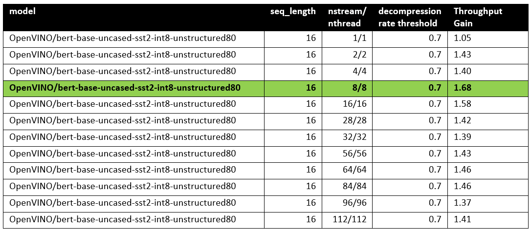
Based on this, we can conclude that one can expect significant performance improvement with any number of streams/threads larger than one. The optimal performance is achieved at eight streams/threads. However, we would like to note that this is model specific and depends on the model architecture and sparsity distribution.
The chart below also shows the relationship between the possible acceleration and the sequence length.
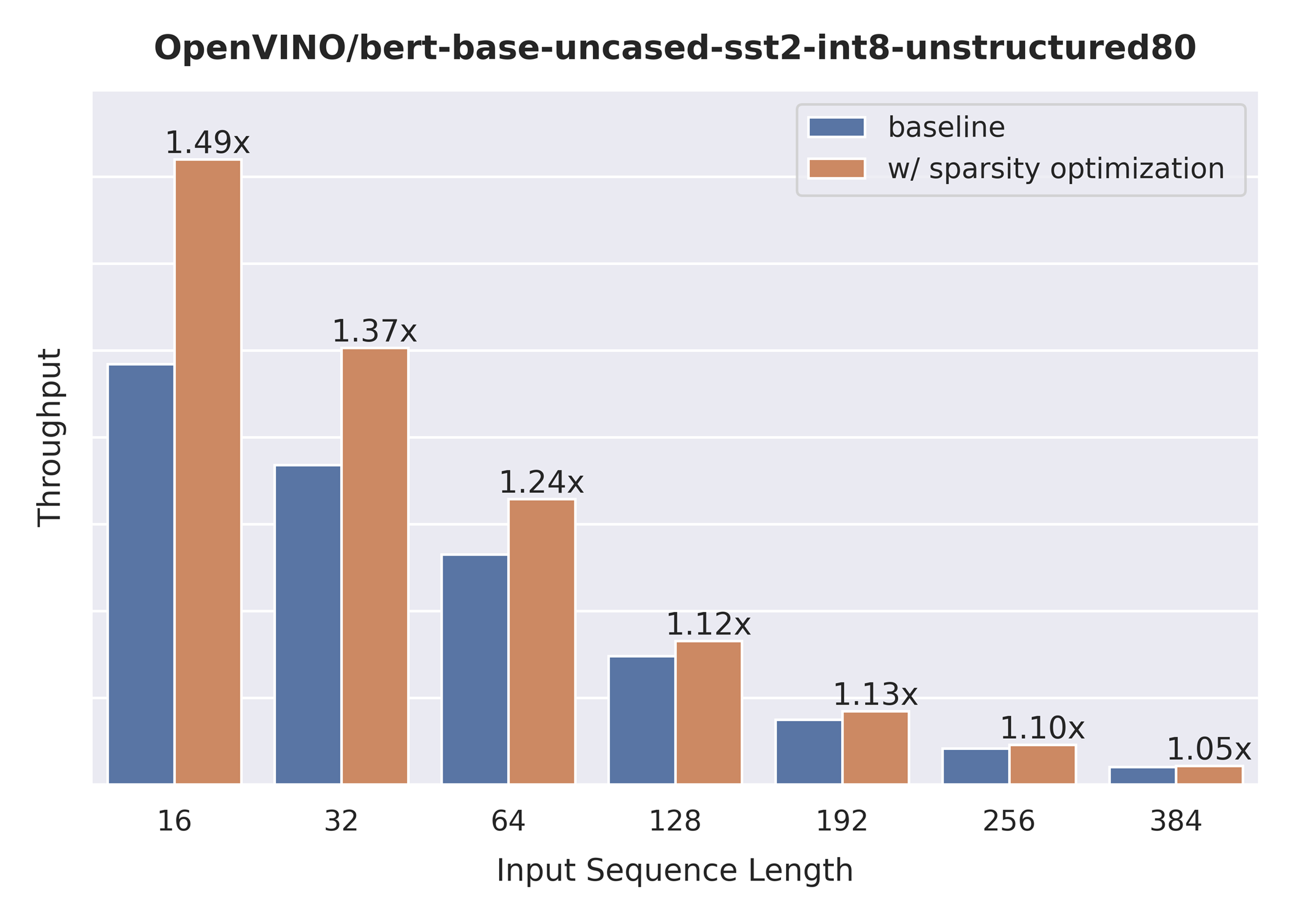
As you can see the benefit from sparsity is decreasing with the growth of the sequence length processed by the model. This effect can be explained by the fact that for larger sequence lengths the size of the weights is no longer a performance bottleneck and weight compression does not have so much impact on the inference time. It means that such a weight sparsity acceleration feature does not suit well for large text processing tasks but could be very helpful for Question Answering, Sequence Classification, and similar tasks.
Authors: Ivan Novoselov, Alexandra Sidorova, Vladislav Golubev, Dmitry Gorokhov
Introduction
Deep learning (DL) has become a powerful tool for addressing challenges in various domains like computer vision, generative AI, and natural language processing. Industrial applications of deep learning often require performing inference in resource-constrained environments or in real time. That’s why it’s essential to optimize inference of DL models for particular use cases, such as low-latency, high-throughput or low-memory environments. Thankfully, there are several frameworks designed to make this easier, and OpenVINO stands out as a powerful tool for achieving these goals.
OpenVINO is an open-source toolkit for optimization and deployment of DL models. It demonstrates top-tier performance across a variety of hardware including CPU (x64, ARM), AI accelerators (Intel NPU) and Intel GPUs. OpenVINO supports models from popular AI frameworks and delivers out-of-the box performance improvements for diverse applications (you are welcome to explore demo notebooks). With ongoing development and a rapidly growing community, OpenVINO continues to evolve as a versatile solution for high-performance AI deployments.
The primary objective of OpenVINO is to maximize performance for a given DL model. To do that, OpenVINO applies a set of hardware-dependent optimizations The optimizations are typically performed by replacing a target group of operations with a custom operation that can be executed more efficiently. In the standard approach, these custom operations are executed using handcrafted implementations. This approach is highly effective when optimizing a few patterns of operations. On the other hand, it lacks scalability and thus requires too much effort when dozens of similar patterns should be supported.
To address this limitation and build a more flexible optimization engine, OpenVINO introduced Snippets, an integrated Just-In-Time (JIT) compiler for computational graphs. Snippets provide a flexible and scalable approach for operation fusions and enablement. The graph compiler automatically identifies subgraphs of operations that can benefit from fusion and combines them into a single node, referred to as “Subgraph”. Snippets then apply a series of optimizing transformations to the subgraph and JIT compile an executable that efficiently performs the computations defined by the subgraph.
One of the most common examples of such subgraphs is Scaled Dot-Product Attention (SDPA) pattern. SDPA it is a cornerstone of transformer-based architectures which dominate most of the state-of-the-art models. There are numerous SDPA pattern flavours and variations dictated by model-specific adjustments or optimizations. Thanks to compiler-based design, Snippets support most of these configurations. Fig. 1 illustrates the general structure of the SDPA pattern supported by Snippets, highlighting its adaptability to different model requirements:
Figure 1. SPDA variations supported by Snippets. Blocks with a dashed border denote optional operations. The operations listed inside the block can be in any order. The semantics of the operations are described in the OpenVINO documentation.
Note that SDPA has quadratic time and memory complexity with respect to sequence length. It means that by fusing SDPA-like patterns, Snippets significantly reduce memory consumption and accelerate transformer models, especially for large sequence lengths.
Snippets effectively optimized SDPA patterns but had a key limitation: they did not support dynamic shapes. In other words, input shapes must be known at the model compilation stage and can’t be changed in runtime. This limitation reduced the applicability of Snippets to many real-world scenarios where input shapes are not known in advance. While it is technically possible to JIT-compile a new binary for each unique set of input shapes, this approach introduces significant recompilation overheads, often negating the performance gains from SDPA fusion.
Fortunately, this static-shape limitation is not inherent to Snippets design. They can be modified to support dynamic shapes internally and generate shape-agnostic binaries. In this post, we discuss Snippets architecture and the challenges we faced during this dynamism enablement.
Architecture
The first step of the Snippets pipeline is called Tokenization. It is applied to an ov::Model, which represents OpenVINO Intermediate Representation (IR). It’s a standard IR in the OV Runtime you can read more about it here or here. The purpose of this stage is to identify parts of the initial model that can be lowered by Snippets efficiently. We are not going to discuss Tokenization in detail because this article is mostly focused on the dynamism implementation. A more in-depth description of the Tokenization process can be found in the Snippets design guide. The key takeaway for us here is that the subsequent lowering is performed on a part of the initial ov::Model. We will call this part Subgraph, and the Subgraph at first is also represented as an ov::Model.
Now let’s have a look at the lowering pipeline, its schematic representation is shown on Fig.2a. As can be seen from the picture, the lowering process consists of three main phases: Data Flow Optimizations, Control Flow Optimizations and Binary Code Generation. Let’s briefly discuss each of them.
Figure 2. Snippets architecture. a) — lowering pipeline view, b) — a closer look at shape-sensitive stages, c) — dynamic pipeline implementation scheme.
Lowering Pipeline
The first stage is the Data Flow optimizations. As we mentioned above, this stage’s input is a part of the initial model represented as an ov::Model. This representation is very convenient for high-level transformations such as opset conversion, operations’ fusion/decomposition and precision propagation. Here are some examples of the transformations performed on this stage:
ConvertPowerToPowerStatic — operation Power with scalar exponent input is converted to PowerStatic operation from the Snippets opset. The PowerStatic ops then use the values of the exponents to produce more optimal code.
FuseTransposeBrgemm — Transpose operations that can be executed in-place with Brgemm blocks are fused into the Brgemm operations.
PrecisionPropagation pass automatically inserts Converts operations between the operations that don’t natively support the desired execution precision.
The next stage of the lowering process is Control Flow optimizations (or simply CFOs). Note that the ov::Model is designed to primarily describe data flow, so is not very convenient for CFOs. Therefore, we had to develop our own IR (called Linear IR or simply LIR) that explicitly represents both control and data flows, you can read more about LIR here. So the ov::Model IR is converted to LIR before the start of the CFOs.
As you can see from the Fig.2a, the Control Flow optimization pipeline could roughly be divided into three main blocks. The first one is called Loop Generation and Optimization. This block includes all loop-related optimizations such as automatic generation of loops based on the input tensors’ dimensions, loop fusion and blocking loops generation.
The second block of Control Flow optimizations is called Utility Ops Insertion. We need this block of transformations here to insert utility operations that depend on loop control structures, specifically on their entry and exit points locations. For example, operations like Load, Store, MemoryBuffer, LoopBegin and LoopEnd are inserted during this stage.
The last step of CFO is the Memory Usage Optimizations block. These transformations determine required sizes of internal memory buffers, and analyze how much of that memory can be reused. A graph coloring algorithm is employed to minimize memory consumption.
Now all Control Flow optimizations are performed, and we are ready to proceed to the next stage of the lowering pipeline — Binary Code Generation (BCG). As one can see from Fig.2a, this stage consists of three substages. The first one is Register Assignment. We use a fairly standard approach here: calculate live intervals first and use the linear scan algorithm to assign abstract registers that are later mapped to physical ones.
The next BSG substage is Loop Expansion. To better understand its purpose, let’s switch gears for a second and think about loops in general. Sometimes it’s necessary to process the first or the last iteration of a loop in a special way. For example, to initialize a variable or to process blocking loops’ tails. The Loop Expansion pass unrolls these special iterations (usually the first or the last one) and explicitly injects them into the IR. This is needed to facilitate subsequent code emission.
The final step of the BCG stage is Code Emission. At this stage, every operation in our IR is mapped to a binary code emitter, which is then used to produce a piece of executable code. As a result, we produce an executable that performs calculations described by the initial input ov::Model.
Dynamic Shapes Support
Note that some stages of the lowering pipeline are inherently shape-sensitive, i.e. they rely on specific values of input shapes to perform optimizations. These stages are schematically depicted on the Fig. 2b.
As can be seen from the picture, shapes are used to determine loops’ work amounts and pointer increments that should be performed on every iteration. These parameters are later baked into the executable during Code Emission. Another example is Memory Usage Optimizations, since input shapes are needed to calculate memory consumption. Loop Expansion also relies on input shapes, since it needs to understand if tail processing is required for a particular loop. Note also that Snippets use compute primitives from third-party libraries, BRGEMM block from OneDNN for example. These primitives should as well be compiled with appropriate parameters that are also shape-sensitive.
One way to address these challenges is to rerun the lowering pipeline for every new set of input shapes, and to employ caching to avoid processing the same shapes twice. However, preliminary analysis indicated that this approach is too slow. Since this re-lowering needs to be performed in runtime, the performance benefit provided by Snippets is essentially eliminated by the recompilation overheads.
The performed experiments thus indicate that we can afford to run the whole lowering pipeline only once during the model compilation stage. Only some minor adjustments can be made at runtime. In other words, we need to remove all shape-sensitive logic from the lowering pipeline and perform the compilation without it. The remaining shape-sensitive transformations should be performed at runtime. Of course, we would also need to share this runtime context with the compiled shape-agnostic kernel. The idea behind this approach is schematically represented on Fig. 2c.
As one can see from the picture, all the shape-sensitive transformations are now performed by a new entity called Runtime Configurator. It’s probably easier to understand its purpose in some examples.
Imagine that we need to perform a unary operation get_result(X) on an input tensor X — for example, apply an activation function. To do this, we need to load some input data from memory into registers, perform the necessary computations and write the results back to memory. Of course this read-compute-write sequence should be done in a loop since we need to process the entire input tensor. These steps are described in more detail in Fig. 3 using pseudocode. Fig. 3a corresponds to a static kernel while Fig. 3b represents a dynamic one.
Let’s consider the static kernel as a starting point. As the first step, we need to load pointers to input and output memory blobs to general-purpose registers (or simply GPRs) denoted G_IN and G_OUT on the picture. Then we initialize another GPR that stores the loop work amount (G_WA). Note that the loop is used to traverse the input tensor, so the loop’s work amount is fixed because the tensor’s dimensions are also known at the BCG stage. The next six steps in the picture (3 to 8) are in the loop’s body.
Figure 3. Pseudocode for performing an unary operation “get_result” for a) — static and b) — dynamic kernels. Note that general-purpose and vector registers are denoted with “G_” and “V_” prefixes, respectively.
In step 3, we load input data into a vector register V_0, note that the appropriate pointer is already loaded to G_IN, and offset_in is fixed because the input tensor is static. Next, we apply our get_result function to the data in V_0 and place the result in a spare vector register V_1. Now we need to store V_1 back to memory, which is done on step 5. Note that offset_out is also known in the static case. This brings us almost to the end of the loop’s body, and the last few things we need to do are to increment data pointers (step 6), decrement loop counter (step 7), and jump to the beginning of the body, if needed (step 8).
Finally, we need to reset data pointers to their initial values after the loop is finished, which is done using finalization offsets on step 9. Note that this step could be omitted in our simplified example, but it’s often needed for more complicated use cases, such as when the data pointers are used by subsequent loops.
Now that we understand the static kernel, let’s consider the dynamic one, which is shown in Fig. 3b. Unsurprisingly, the dynamic kernel performs essentially the same steps as the static one, but with additional overhead due to loading shape-dependent parameters from the extended runtime arguments. Take step 1 as an example, we need to load not only memory pointers (to G_IN and G_OUT), but also a pointer to the runtime arguments prepared by the runtime configurator (to G_ARG).
Next, we need to load a pointer to the appropriate loop descriptor (a structure that stores loops’ parameters) to a temporary register G_TMP, and only then we can initialize the loop’s work amount register G_WA (step 2). Similarly, in order to load data to V_0, we need to load a runtime-calculated offset from the runtime arguments in step 3. The computations in step 4 are the same as in the static case, since they don’t depend on the input shapes. Storing the results to memory (step 5) requires reading a dynamic offset from the runtime arguments again. Next, we need to shift the data pointers, and again we have to load the increments from the corresponding loop descriptor in G_ARG because they are also shape-dependent, as the input tensor can be strided. The following two steps 7 and 8 are the same as in the static case, but the finalization offsets are also dynamic, so we have to load them from G_ARG yet again.
As one can see from Fig. 3, dynamic kernels incorporate additional overhead due to reading the extended runtime parameters provided by the runtime configurator. However, this overhead could be acceptable as long as the input tensor is large enough (Load/Store operations would take much longer than reading runtime arguments from L1) and the amount of computation is sufficient (get_results is much larger than the overhead). Let’s consider the performance of this design in the Results section to see if these conditions are met in practical use cases.
Results
We selected three platforms to evaluate the dynamic pipeline’s performance in Snippets. These platforms represent different market segments: the Intel Core machine is designed for high-performance user and professional tasks. While the Intel Xeon is a good example of enterprise-level hardware often used in data centers and cloud computing applications. The information about the platforms is described in the table below:
As discussed in the Introduction, Snippets support various SDPA-like patterns which form the backbone of Transformer models. These models often work with input data of arbitrary size (for example, sequence length in NLP). Thus, dynamic shapes support in Snippets can efficiently accelerate many models based on Transformer architecture with dynamic inputs.
We selected 43 different Transformer-models from HuggingFace to measure how the enablement of dynamic pipeline in Snippets affects performance. The models were downloaded and converted to OpenVINO IRs using Optimum Intel. These models represent different domains and were designed to solve various tasks in natural language processing, text-to-image image generation and speech recognition (see full model list at the end of the article). What unifies all these models is that they all contain SDPA subgraph and thus can be accelerated by Snippets.
Let’s take a closer look at the selected models. The 37 models of them solve different tasks in natural language processing. Their performance was evaluated using a list of 2000 text sequences with different lengths, which also mimics the real-word scenario. The total processing time of all the sequences were measured in every experiment. Note that the text sequences were converted to model inputs using model-specific tokenizers prior to the benchmarking. The lengths’ distribution of the tokenized sequences is shown on Fig. 4. As can be seen from the picture, the distribution is close to normal with the mean length of 31 tokens.
Figure 4. Distribution of input prompt lengths that were used for benchmarking of NLP models. Vertical dashed line denotes the mean of the distribution.
The other 6 models of the selected model scope solve tasks in text-to-image image generation (Stable Diffusion) and speech recognition (Whisper). These models decompose into several smaller models after export to OpenVINO representation using Optimum Intel. Stable Diffusion topology is decomposed into Encoder, Diffuser and Decoder. The most interesting model here is Diffuser because it’s the one responsible for denoising of the latent image representation. This generation stage is repeated several times, so it is the most computationally intensive, which mostly effects on the generation time of the image. Whisper is also decomposed into Encoder and Decoder, which also contain SDPA patterns. The Encoder encodes the spectrogram from the feature extractor to form a sequence of encoder hidden states. Then, the decoder autoregressively predicts text tokens, conditional on both the previous tokens and the encoder hidden states. Currently, Snippets support efficient execution of SDPA only in Whisper Encoder, while Decoder is a subject for future support. To evaluate the inference performance of Stable Diffusion and Whisper models, we collect generation time of image/speech using LLM Benchmark from openvino.genai. This script provides a unified approach to estimate performance for GenAI workloads in OpenVINO.
Performance Improvements
Note that the main goal of these experiments is to estimate the impact of Snippets on the performance of the dynamic pipeline. To do that, we performed two series of experiments for every model. The first version of experiments is with disabled Snippets tokenization. In this case, all operations from the SDPA pattern are performed on the CPU plugin side as stand-alone operations. The second variant of experiments — with enabled Snippets tokenization. The relative difference between numbers collected on these two series of experiments is our performance metric — speedup, the higher the better. Firstly, let’s take a closer look at the resulting speedups for the BERT models which are depicted on Fig. 5.
Figure 5. Impact of Snippets enablement on the performance of BERT-models. Vertical dashed lines denote mean values similar to Fig.4.
The speedups on RPL range from 3 to 18%, while on average the models are accelerated by 7%. The ARL-S speedups are somewhat higher and reach 20–25% for some models, the average acceleration factor is around 9%. The most affected platform is SPR, it has the highest average speedup of 15 %.
One can easily see from these numbers that both average and maximum speedups depend on the platform. To understand the reason for this variation, we should recall that the main optimizations delivered by Snippets are vertical fusion and tiling. These optimizations improve cache locality and reduce the memory access overheads. Note SPR has the largest caches among the examined platforms. It also uses BF16 precision that takes two times less space per data element compared to F32 used on ARL-S and RPL. Finally, SPR has AMX ISA extension that allows it to perform matrix multiplications much faster. As a result, SDPA execution was more memory bound on SPR, so this platform benefited the most from the Snippets enablement. At the same time, the model speedups on ARL-S and RPL are almost on the same level. These platforms use FP32 inference precision while SPR uses BF16, and they have less cache size than SPR.
Figure 6. Impact of Snippets enablement on the performance of Stable Diffusion and Whisper models
Now, let’s consider Stable Diffusion and Whisper topologies and compare their speedups with some of BERT-like models. As can be seen from the Fig. 6, the most accelerated Stable Diffusion topology is StableDiffusion-3-medium — almost 33% on ARL-S and 40% on SPR. The most accelerated model in this Stable Diffusion pipeline is Diffuser. This model has made a great contribution to speeding up the entire image generation time. The reason the Diffuser benefits more from Snippets enablement is that they use larger sequence lengths and embedding sizes. It means that their attention blocks process more data and are more memory constrained compared to BERT-like models. As a result, the Diffuser models in Stable Diffusion benefit more from the increased cache locality provided by Snippets. This effect is more pronounced on the SPR than on the ARL-S and RPL for the reasons discussed above (cache sizes, BF16, AMX).
The second most accelerated model is whisper-large-v3–30% on SPR. This model has more parameters than base and tiny models and process more Mel spectrogram frequency bins than they. It means that Encoder of whisper-large-v3 attention blocks processes more data, like Diffuser part of Stable Diffusion topologies. By the same reasons, whisper-large-v3 benefits more (increased cache locality provided by Snippets).
Memory Consumption Improvements
Another important improvement from Snippets using is reduction of memory consumption. Snippets use vertical fusion and various optimizations from Memory Usage Optimizations block (see the paragraph “Lowering Pipeline” in “Architecture” above for more details). Due to this fact, Subgraphs tokenized by Snippets consumes less memory than the same operations performed as stand-alone in CPU Plugin.
Figure 7. Impact of Snippets enablement on the memory consumption of image generation using Stable Diffusion models.
Let’s take a look at the Fig. 7 where we can see improvements in image generation memory consumption using Stable Diffusion pipelines from Snippets usage. As discussed above, the attention blocks in the Diffuser models from these pipelines process more data and consume more memory. Because of that, the greatest impact on memory consumption from using Snippets is seen on Stable Diffusion pipelines. For example, memory consumption of image generation is reduced by 25–50% on RPL and ARL-S platforms with FP32 inference precision and by 15–30% on SPR with BF16 inference precision.
Thus, one of the major improvements from using Snippets is memory consumption reduction. It allows extending the range of platforms which are capable to infer such memory-intensive models as Stable Diffusion.
Conclusion
Snippets is a JIT compiler used by OpenVINO to optimize performance-critical subgraphs. We briefly discussed Snippets’ lowering pipeline and the modifications made to enable dynamism support. After these changes, Snippets generate shape-agnostic kernels that can be used for various input shapes without recompilation.
This design was tested on realistic use cases across several platforms. As a result, we demonstrate that Snippets can accelerate BERT-like models by up to 25%, Stable Diffusion and Whisper pipelines up to 40%. Additionally, Snippets can significantly reduce memory consumption by several tens of percent. Notably, these improvements result from more optimal hardware utilization, so the models’ accuracy remains unaffected.
Performance varies by use, configuration, and other factors. Learn more on the Performance Index site.
No product or component can be absolutely secure. Your costs and results may vary. Intel technologies may require enabled hardware, software or service activation.
The integration of Ollama and OpenVINO delivers a powerful dual-engine solution for the management and inference of large language models (LLMs). Ollama offers a streamlined model management toolchain, while OpenVINO provides efficient acceleration capabilities for model inference across Intel hardware (CPU/GPU/NPU). This combination not only simplifies the deployment and invocation of models but also significantly enhances inference performance, making it particularly suitable for scenarios demanding high performance and ease of use.
You can find more information on github repository:
1. Streamlined LLM Management Toolchain: Ollama provides a user-friendly command-line interface, enabling users to effortlessly download, manage, and run various LLM models.
2. One-Click Model Deployment: With simple commands, users can quickly deploy and invoke models without complex configurations.
3. Unified API Interface: Ollama offers a unified API interface, making it easy for developersto integrate into various applications.
4. Active Open-Source Community: Ollama boasts a vibrant open-source community, providing users with abundant resources and support.
Limitations of Ollama
Currently, Ollama only supports llama.cpp as itsbackend, which presents some inconveniences:
1. Limited Hardware Compatibility: llama.cpp is primarily optimized for CPUs and NVIDIA GPUs, and cannot fully leverage the acceleration capabilities of Intel GPUs or NPUs, resulting in suboptimal performance in high-performance computing scenarios.
2.Performance Bottlenecks: For large-scale models or high-concurrency scenarios, the performance of llama.cpp may fall short, especially when handling complex tasks, leading to slower inference speeds.
Breakthrough Capabilities of OpenVINO
1. Deep Optimization for Intel Hardware (CPU/iGPU/Arc dGPU/NPU): OpenVINO is deeply optimized for Intel hardware, fully leveraging the performance potential of CPUs, iGPUs, dGPUs, and NPUs.
2. Cross-Platform Heterogeneous Computing Support: OpenVINO supports cross-platform heterogeneous computing, enabling efficient model inference across different hardware platforms.
3. Model Quantization and Compression Toolchain: OpenVINO provides a comprehensive toolchain for model quantization and compression, significantly reducing model size and improving inference speed.
4. Significant Inference Performance Improvement: Through OpenVINO's optimizations, model inference performance can be significantly enhanced, especially for large-scale models and high-concurrency scenarios.
5. Extensibility and Flexibility Support: OpenVINO GenAI offers robust extensibility and flexibility for Ollama-OV, supporting pipeline optimization techniques such as speculative decoding, prompt-lookup decoding, pipeline parallelization, and continuous batching, laying a solid foundation for future pipeline serving optimizations.
Developer Benefits of Integration
1.Simplified Development Experience: Retains Ollama's CLI interaction features, allowing developers to continue using familiar command-line tools for model management and invocation.
2.Performance Leap: Achieves hardware-level acceleration through OpenVINO, significantly boosting model inference performance, especially for large-scale models and high-concurrency scenarios.
3.Multi-Hardware Adaptation and Ecosystem Expansion: OpenVINO's support enables Ollama to adapt to multiple hardware platforms, expanding its application ecosystem and providing developers with more choices and flexibility.
For Windows systems, first extract the downloaded OpenVINO GenAI package to the directory openvino_genai_windows_2025.2.0.0.dev20250320_x86_64, then execute the following commands:
cd openvino_genai_windows_2025.2.0.0.dev20250320_x86_64
setupvars.bat
3. Set Up cgocheck
Windows:
set GODEBUG=cgocheck=0
Linux:
export GODEBUG=cgocheck=0
At this point, the executable files have been downloaded, and the OpenVINO GenAI, OpenVINO, and CGO environments have been successfully configured.
Custom Model Deployment Guide
Since the Ollama Model Library does not support uploading non-GGUF format IR models, we will create an OCI image locally using OpenVINO IR that is compatible with Ollama. Here, we use the DeepSeek-R1-Distill-Qwen-7B model as an example:
With these steps, we have successfully created the DeepSeek-R1-Distill-Qwen-7B-int4-ov:v1 model, which is now ready for use with the Ollama OpenVINO backend.
Alexander Kozlov, Nikolay Lyalyushkin, Nikita Savelyev, Souvikk Kundu, Andrey Anufriev, Pablo Munoz, Alexander Suslov, Liubov Talamanova, Daniil Lyakhov, Yury Gorbachev, Nilesh Jain, Maxim Proshin, Evangelos Georganas
Summary
This quarter we noticed a significant effort and progress on optimizing LLMs for long-context tasks. The current trend is that each and every LLM is published with the extended (usually interpolated) context which is usually 128K and above. The idea is to naturally process large amount of data within the model instead of preprocess it the way RAG systems do it. It inevitably increases computational complexity specifically of ScaledDotProductAttention operation which gets dominant on long contexts. Thus, many works devoted to the optimization of rather prefill with special computation patterns (A-shape, Tri-shape, XAttention) or using Sparse Attention at the decoding stage.
Highlights
ParetoQ: Scaling Laws in Extremely Low-bit LLM Quantization by Meta (https://arxiv.org/pdf/2502.02631). The paper presents a unified framework that facilitates comparisons across 1-bit, 1.58-bit, 2-bit, 3-bit, and 4-bit quantization settings. The findings reveal a notable learning transition between 2 and 3 bits: For 3-bits and above, the fine-tuned models stay close to their original pre-trained distributions, whereas for learning 2-bit networks or below, the representations change drastically. By optimizing training schemes and refining quantization functions, the ternary 600M-parameter model even outperforms the previous SoTA ternary 3B-parameter model in accuracy, using only one-fifth of the parameters.
QuEST: Stable Training of LLMs with 1-Bit Weights and Activations by ISTA and Red Hat AI (https://arxiv.org/pdf/2502.05003). The paper introduces quantization method that allows stable training with 1-bit weights and activations. It achieves this by improving two key aspects of QAT methods: (1) accurate and fast quantization of the (continuous) distributions of weights and activations via Hadamard normalization and MSE-optimal fitting; (2) a new trust gradient estimator based on the idea of explicitly minimizing the error between the noisy gradient computed over quantized states and the “true” (but unknown) full-precision gradient. Experiments on Llama-type architectures show that the method induces stable scaling laws across the entire range of hardware-supported precisions, and can be extended to sparse representations. The code is available at https://github.com/IST-DASLab/QuEST.
Native Sparse Attention: Hardware-Aligned and Natively Trainable Sparse Attention by Deepseek-AI, Peking University, University of Washington (https://arxiv.org/pdf/2502.11089). The paper presents a method with hardware-aligned optimizations to achieve efficient long-context modeling. It employs a dynamic hierarchical sparse strategy, combining coarse-grained token compression with fine-grained token selection to preserve both global context awareness and local precision. The approach advances sparse attention design with two key features: (1) Authors achieve substantial speedups through arithmetic intensity-balanced algorithm design, with implementation optimizations for modern hardware. (2) They enable end-to-end training, reducing pretraining computation without sacrificing model performance. Experiments show the model pretrained with the proposed method maintains or exceeds Full Attention models across general benchmarks, long-context tasks, and instruction-based reasoning. It achieves substantial speedups over Full Attention on 64k-length sequences across decoding, forward propagation, and backward propagation. Non-official implementations are available on GitHub.
LSERVE: EFFICIENT LONG-SEQUENCE LLM SERVING WITH UNIFIED SPARSE ATTENTION by MIT, SJTU, Nvidia (https://arxiv.org/pdf/2502.14866). The paper introduces a system that accelerates long-sequence LLM serving via hybrid sparse attention. This method unifies different hardware-friendly, structured sparsity patterns for both prefilling and decoding attention into a single framework, where computations on less important tokens are skipped block-wise. It demonstrates the compatibility of static and dynamic sparsity in long-context LLM attention. Authors convert half of the attention heads to nearly free streaming heads in both the prefilling and decoding stages. Additionally, we they that only a constant number of KV pages is required to preserve long-context capabilities, irrespective of context length. They then design a hierarchical KV page selection policy that dynamically prunes KV pages based on query-centric similarity. The method accelerates LLM prefilling by up to 2.9x and decoding by 1.3-2.1x over vLLM, maintaining long-context accuracy. Code is released at https://github.com/mit-han-lab/omniserve.
XAttention: Block Sparse Attention with Antidiagonal Scoring by Tsinghua University, MIT, SJTU, and NVIDIA (https://arxiv.org/pdf/2503.16428). The paper introduces XAttention method that significantly accelerates long-context inference in Transformers models using sparse attention. XAttention’s key innovation is the insight that the sum of antidiagonal values (i.e., from the lower-left to upper-right) in the attention matrix provides a powerful proxy for block importance. This allows for precise identification and pruning of non-essential blocks, resulting in high sparsity and dramatically accelerated inference. On RULER and LongBench for language, VideoMME for video understanding, and VBench for video generation—XAttention achieves accuracy comparable to full attention while delivering substantial computational gains. It shows up to 13.5x acceleration in attention computation. The code is available at https://github.com/mit-han-lab/x-attention.
Papers with notable results
Quantization
Optimizing Large Language Model Training Using FP4 Quantization by Microsoft and University of Science and Technology of China (https://arxiv.org/pdf/2501.17116). The work introduces the FP4 training framework for LLMs, addressing quantization challenges with two key ideas: a differentiable quantization estimator for precise weight updates and an outlier clamping and compensation strategy to prevent activation collapse. To ensure stability, the framework integrates a mixed-precision training scheme and vector-wise quantization. Experimental results demonstrate that our FP4 framework achieves accuracy comparable to BF16 and FP8, with minimal degradation, scaling effectively to 13B-parameter LLMs trained on up to 100B.
MQuant: Unleashing the Inference Potential of Multimodal Large Language Models via Full Static Quantization by Houmo AI, Southeast University, and Xi’an Jiaotong University (https://arxiv.org/pdf/2502.00425). The work focuses on the problems of VLM quantization with a coarse scale granularity. It proposes several techniques to tackle the quantization problems, namely: Modality-Specific Static Quantization (MSQ), assigning distinct static scales for visual vs. textual tokens; Attention-Invariant Flexible Switching (AIFS), reordering tokens to preserve casual attention while eliminating expensive token-wise scale computations; Rotation Magnitude Suppression (RMS), mitigating weight outliers arising from online Hadamard rotations. On five mainstream VLMs (including Qwen-VL, MiniCPM-V, CogVLM2), the method achieves near-floating-point accuracy under W4A8 setting. The code is planned to be published.
An Empirical Study of LLaMA3 Quantization: From LLMs to MLLMs by The University of Hong Kong, Beihang University, and ETH Zurich (https://arxiv.org/pdf/2404.14047). Authors assessed the performance of the LLaMA3-based LLaVA-Next-8B model under 2-4 ultra-low bits with post-training quantization methods. Experimental results indicate that LLaMA3 still suffers from non-negligible degradation in linguistic and visual contexts, particularly under ultra-low bit widths. This highlights the significant performance gap at low bit-width that needs to be addressed in future developments. The code is available at: https://github.com/Macaronlin/LLaMA3-Quantization.
Nanoscaling Floating-Point (NxFP): NanoMantissa, Adaptive Microexponents, and Code Recycling for Direct-Cast Compression of Large Language Models by Harvard University (https://arxiv.org/pdf/2412.19821). This paper profiles modern LLMs and identifies three main challenges of low-bit Microscaling format, i.e., inaccurate tracking of outliers, vacant quantization levels, nd wasted binary code. In response, Nanoscaling (NxFP) proposes three techniques, i.e., NanoMantissa, Adaptive Microexponent, and Code Recycling to enable better accuracy and smaller memory footprint than state-of-the-art MxFP. Experimental results on direct-cast inference across various modern LLMs demonstrate that the proposed methods outperform MxFP by up to 0.64 in perplexity and by up to 30% in accuracy on MMLU benchmarks.
RoSTE: An Efficient Quantization-Aware Supervised Fine-Tuning Approach for Large Language Models by University of Minnesota and The Chinese University of Hong Kong (https://arxiv.org/pdf/2502.09003). The paper introduces a fine-tuning based method that directly optimizes quantized weights and rotation matrices within a single model architecture. It proposes a bilevel optimization formulation, where upper level subproblem optimizes weight matrices, while lower level subproblem employs a surrogate loss to guide the selection of rotation matrix. Authors designed an algorithm which alternates between (i) a QAT subroutine incorporating a rotation-enabled straightthrough-estimator (STE) update, and (ii) a low complexity heuristic for selecting rotation matrices based on the random Walsh-Hadamard matrix. They provide a theoretical analysis of the benefits of rotation-enabled quantization in QA-SFT by examining the prediction error resulted from the QAT stage of RoSTE. This analysis directly motivates the use of quantization error based surrogate loss and justifies the adoption.
NESTQUANT: NESTED LATTICE QUANTIZATION FOR MATRIX PRODUCTS AND LLMS by MIT and Hebrew University of Jerusalem (https://arxiv.org/pdf/2502.09720). The paper proposes a PTQ scheme for weights and activations that is based on self-similar nested lattices. Recent work has mathematically shown such quantizers to be information-theoretically optimal for low-precision matrix multiplication. We implement a practical low-complexity version based on Gosset lattice, making it a drop-in quantizer for any matrix multiplication step (e.g., in self-attention, MLP etc). For example, the method quantizes weights, KV-cache, and activations of Llama-3-8B to 4 bits, achieving perplexity of 6.6 on wikitext2.
ViM-VQ: Efficient Post-Training Vector Quantization for Visual Mamba by Zhejiang University and vivo Mobile (https://arxiv.org/pdf/2503.09509). A practical study of vector quantization method for Visual Mamba networks (ViMs). Authors identify several key challenges: 1) The weights of Mamba-based blocks in ViMs contain numerous outliers, significantly amplifying quantization errors. 2) When applied to ViMs, the latest VQ methods suffer from excessive memory consumption, lengthy calibration procedures, and suboptimal performance in the search for optimal codewords. They propose a post-training vector quantization method tailored for ViMs. It consists of two components: 1) a fast convex combination optimization algorithm that updates both the convex combinations and the convex hulls to search for optimal codewords, and 2) an incremental vector quantization strategy that incrementally confirms optimal codewords to mitigate truncation errors. The results demonstrate that the method achieves stateof-the-art performance in low-bit quantization across various visual tasks.
SSVQ: Unleashing the Potential of Vector Quantization with Sign-Splitting by Zhejiang University and vivo Mobile (https://arxiv.org/pdf/2503.08668). The paper proposes the vector quantization approach which decouples the sign bit of weights from the codebook. It involves extracting the sign bits of uncompressed weights and performing clustering and compression on all-positive weights. Authors also introduce latent variables for the sign bit and jointly optimize both the signs and the codebook. Additionally, they implement a progressive freezing strategy for the learnable sign to ensure training stability. Experiments on modern models and tasks demonstrate that the method achieves a good compression-accuracy trade-off compared to conventional VQ. Authors also validate the algorithm on a hardware accelerator, showing that SSVQ achieves a 3× speedup over the 8-bit compressed model by reducing memory access.
MergeQuant: Accurate 4-bit Static Quantization of Large Language Models by Channel-wise Calibration (https://arxiv.org/pdf/2503.07654). The paper introduces per-channel static quantization method. It integrates the per-channel quantization steps with the corresponding scalings and linear mappings through a Quantization Step Migration method, eliminating the quantization overheads before and after matrix multiplication. Authors also propose dimensional reconstruction and adaptive clipping to address the nonuniformity of quantization scale factors and redistribute the channel variations to the subsequent modules to balance the parameter distribution under QSM. They evaluate method on Llama 2 and Llama 3 models in W4A4 setting.
QuantCache: Adaptive Importance-Guided Quantization with Hierarchical Latent and Layer Caching for Video Generation by Shanghai Jiao Tong University, MGTV, Shanhai Academy (https://arxiv.org/pdf/2503.06545). Authors propose a training-free inference acceleration framework that jointly optimizes hierarchical latent caching, adaptive importance-guided quantization, and structural redundancy-aware pruning. It achieves an end-to-end latency speedup of 6.72x on OpenSora with minimal loss in generation quality. experiments across multiple video generation benchmarks demonstrate the effectiveness of our method for DiT inference. The code and models will be available at https://github.com/JunyiWuCode/QuantCache.
Matryoshka Quantization by Google DeepMind (https://arxiv.org/pdf/2502.06786). Practitioners are often forced to maintain multiple models with different quantization levels or serve a single model that best satisfies the quality-latency trade-off. On the other hand, integer data types, such as int8, inherently possess a nested (Matryoshka) structure where smaller bit-width integers, like int4 or int2, are nested within the most significant bits. In this paper, the authors propose Matryoshka Quantization (MatQuant), a multi-scale quantization technique that alleviates the aforementioned challenge. It allows us to train and maintain a single quantized model but serve it with the precision demanded by the deployment. Furthermore, leveraging MatQuant’s co-training and co-distillation regularization, int2 precision models extracted by MatQuant outperform standard int2 quantization by up to to 4% and 7% with OmniQuant and QAT as base algorithms respectively. Finally, authors demonstrate that by using an extra bit to represent outliers, a model with an effective precision of 2.05-bit gives an additional 6% improvement with OmniQuant as the base algorithm.
Pruning/Sparsity
Mamba-Shedder: Post-Transformer Compression for Efficient Selective Structured State Space Models by Intel Labs (https://arxiv.org/pdf/2501.17088v1). This paper explores the compression of SSM-based models, particularly Mamba and its hybrids. The authors discuss the sensitivity of these models to the removal of selected components at different granularities to reduce the model size and computational overhead, thus improving their efficiency while maintaining accuracy. The proposed solutions, collectively referred to as Mamba-Shedder, achieve a speedup of up to 1.4x during inference, demonstrating that model efficiency can be improved by eliminating several redundancies with minimal impact on the overall model performance. The code is available at https://github.com/IntelLabs/Hardware-Aware-Automated-Machine-Learning.
Qwen2.5-1M Technical Report by Alibaba (https://qianwen-res.oss-cn-beijing.aliyuncs.com/Qwen2.5-1M/Qwen2_5_1M_Technical_Report.pdf). Authors introduce Qwen2.5-1M, a series of models that extend the context length to 1 million tokens. Compared to the previous 128K version, the Qwen2.5-1M series has significantly enhanced long-context capabilities through long-context pretraining and post-training. To reduce inference costs, authors implement a sparse attention method along with chunked prefill optimization for deployment scenarios and a sparsity refinement method to improve precision. Additionally, they detail optimizations in the inference engine, including kernel optimization, pipeline parallelism, and scheduling optimization, which significantly enhance overall inference performance. Qwen2.5-1M models achieve a remarkable 3x to 7x prefill speedup in scenarios with 1 million tokens of context.
WaferLLM: A Wafer-Scale LLM Inference System by University of Edinburgh and Microsoft (https://arxiv.org/pdf/2502.04563). The paper introduces LLM inference system that is guided by a device model that captures the unique hardware characteristics of wafer-scale architectures. It proposes MeshGEMM and MeshGEMV, the GEMM and GEMV implementations designed to scale effectively on wafer-scale accelerator. Authors focus on four principles when designing the implementation: Massive Parallel cores, Highly non-uniform memory access Latency, Constrained local Memory, and Limited hardware-assisted Routing. Evaluations show that the method achieves 200× better wafer-scale accelerator utilization than state-of-the-art systems. On a commodity wafer-scale accelerator, it delivers 606× faster and 22× more energy-efficient GEMV compared to an advanced GPU. One of the limitations of the method is a limited model size due to a need to replicate memory over the computational units to increase the latency.
EmbBERT-Q: Breaking Memory Barriers in Embedded NLP by Politecnico di Milano (https://arxiv.org/pdf/2502.10001). The paper proposes a new LM model specifically designed for tiny devices, combining efficiency and effectiveness. Authors analytically evaluate the memory usage and computational complexity of the model and its components, providing a tool to evaluate the weights and activations of memory trade-offs required to operate within tiny device constraints. They also release all code, scripts, and model checkpoints at https://github.com/RiccardoBravin/tiny-LLM.
M2R2: MIXTURE OF MULTI-RATE RESIDUALS FOR EFFICIENT TRANSFORMER INFERENCE by Apple (https://arxiv.org/pdf/2502.02040). The paper introduce Mixture of Multi-rate Residuals, a framework that dynamically modulates the velocity of residual transformations to optimize early residual alignment. This modification improves inference efficiency by better aligning intermediate representations at earlier stages. Authors show the efficacy of the technique in diverse optimization setups such as dynamic computing, speculative decoding, and MoE Ahead-of-Time. In self-speculative decoding setups, M2R2 achieves up to 2.8X speedups on MT-Bench under lossless conditions. In Mixture-of-Experts architectures, they enhance decoding speed by coupling early residual alignment with ahead-of-time expert loading into high-bandwidth memory. This enables concurrent memory access and computation, reducing the latency bottlenecks inherent in expert switching during decoding. Empirical results show that the method delivers a speedup of 2.9X in MoE architectures.
Extending Language Model Context Up to 3 Million Tokens on a Single GPU by KAIST and DeepAuto.ai (https://arxiv.org/pdf/2502.08910). To enable efficient and practical long-context utilization, authors introduce an LLM inference framework that accelerates processing by dynamically eliminating irrelevant context tokens through a modular hierarchical token pruning algorithm. The method also allows generalization to longer sequences by selectively applying various RoPE adjustment methods according to the internal attention patterns within LLMs. They also offload the key-value cache to host memory during inference, significantly reducing GPU memory pressure. As a result, the method enables the processing of up to 3 million tokens on a single L40s 48GB GPU without any permanent loss of context information. The framework achieves an 18.95x.
KernelBench: Can LLMs Write Efficient GPU Kernels? by Stanford University and Princeton University (https://arxiv.org/pdf/2502.10517). The paper introduces KernelBench, an open-source framework for evaluating LMs’ ability to write fast and correct kernels on a suite of 250 carefully selected PyTorch ML workloads. KernelBench represents a real-world engineering environment and making progress on the introduced benchmark directly translates to faster practical kernels. Auhors introduce a new evaluation metric fastp, which measures the percentage of generated kernels that are functionally correct and offer a speedup greater than an adjustable threshold p over baseline. Experiments across various models and test-time methods show that frontier reasoning models perform the best out of the box but still fall short overall, matching the PyTorch baseline in less than 20% of the cases.
Investigating the Impact of Quantization Methods on the Safety and Reliability of Large Language Models by Skolkovo Institute, Artificial Intelligence Research Institute, HSE University (https://arxiv.org/pdf/2502.15799). Authors introduce OpenSafetyMini, a openended safety dataset designed to better distinguish between models. They evaluate 4 state-ofthe-art quantization techniques across LLaMA and Mistral models using 4 benchmarks, including human evaluations. Findings reveal that the optimal quantization method varies for 4-bit precision, while vector quantization techniques deliver the best safety and trustworthiness performance at 2-bit precision, providing foundation for future research. The dataset and reproduces available at: https://github.com/On-Point-RND/OpenSafetyMini-Investigating-the-Impact-of-Quantization-Methods-on-the-Safety-and-Reliability-of-LLM.
MOBA: MIXTURE OF BLOCK ATTENTION FOR LONG-CONTEXT LLMS by Moonshot AI, Tsinghua University, and Zhejiang University (https://arxiv.org/pdf/2502.13189v1). In this work, authors propose a solution that adheres to the “less structure” principle, allowing the model to determine where to attend autonomously, rather than introducing predefined biases. They introduce Mixture of Block Attention (MoBA), an approach that applies the principles of Mixture of Experts (MoE) to the attention mechanism. It is based on block partitioning and routing strategy within Multi-Head Self-Attention. The code is available at https://github.com/MoonshotAI/MoBA.
JUDGE DECODING: FASTER SPECULATIVE SAMPLING REQUIRES GOING BEYOND MODEL ALIGNMENT by Meta GenAI and ETH Zurich (https://openreview.net/pdf?id=mtSSFiqW6y). The paper demonstrates through a series of experiments how the decision mechanism in speculative decoding rejects many high-quality tokens, identifying a key limitation of the technique. Authors adapt verification using ideas from LLM-as-a-judge, eliciting the same versatile rating capability in the target by adding a simple linear layer that can be trained in under 1.5 hours. Using a Llama 8B/70B-Judge, the proposed approach obtains speedups of 9x over standard decoding, achieving an unprecedented 129 tokens/s, while maintaining the quality of Llama-405B on a range of benchmarks.
Software
FlashMLA by Deepseek: https://github.com/deepseek-ai/FlashMLA. FlashMLA is an efficient MLA decoding kernel for Hopper GPUs, optimized for variable-length sequences serving.
DeepSeek releases DeepGEMM is a library designed for clean and efficient FP8 General Matrix Multiplications (GEMMs) with fine-grained scaling: https://github.com/deepseek-ai/DeepGEMM.