Tuning

Authors: Mingyu Kim, Vladimir Paramuzov, Nico Galoppo

Intel’s newest GPUs, such as Intel® Data Center GPU Flex Series, and Intel® Arc™ GPU, introduce a range of new hardware features that benefit AI workloads. Starting with the 2022.3 release, OpenVINO™ can take advantage of two newly introduced hardware features: XMX (Xe Matrix Extension) and parallel stream execution. This article explains what those features are and how you can check whether they are enabled in your environment. We also show how to benefit from them with OpenVINO, and the performance impact of doing so.

What is XMX (Xe Matrix Extension)?

XMX is a hardware acceleration for matrix multiplication on the newest Intel™ GPUs. Given the same number of Xe Cores, XMX technology provides 4-8x more multiplication capacity at the same precision [1]. OpenVINO, powered by OneDNN, can take advantage of XMX hardware by accelerating int8 and fp16 inference. It brings performance gains in compute-intensive deep learning primitives such as convolution and matrix multiplication.

Under the hood, XMX is a well-known hardware architecture called a systolic array. Systolic arrays increase computational capacity without increasing memory (or register) access. The magic happens by pipelining multiple computations with a single data access, as opposed to the traditional fetch-compute-store pipeline. It is implemented by connecting multiple computation nodes in series. Data is fed into the front, goes through several steps of multiplication-add, and finally is stored back to memory.

How to check whether you have XMX?

You can check whether your GPU hardware (and software stack) supports XMX with OpenVINO™’s hello_query_device sample. When you run the sample application, it lists all detected inference devices along with its properties. You can check for XMX support by looking at the OPTIMIZATION_CAPABILITIES property and checking for the GPU_HW_MATMUL value.

In the listing below you can see that our system has two GPU devices for inference, and only GPU.1 has XMX support.

$ ./hello_query_device
[ INFO ] GPU.0
[ INFO ]        SUPPORTED_PROPERTIES: 
[ INFO ]                Immutable: OPTIMIZATION_CAPABILITIES : FP32 BIN FP16 INT8      
# XMX is not supported
[ INFO ] GPU.1
[ INFO ]        SUPPORTED_PROPERTIES: 
[ INFO ]                Immutable: OPTIMIZATION_CAPABILITIES : FP32 BIN FP16 INT8 GPU_HW_MATMUL    
# XMX is supported

‍

As mentioned, XMX provides a way to get significantly more compute capacity on a GPU. The next feature doesn’t provide more capacity, but it allows ways to use that capacity more efficiently.

What is parallel execution of multiple streams?

Another improvement of Intel®’s discrete GPUs is to process multiple compute streams in parallel. Certain deep learning inference workloads are too small to fill all hardware compute resources of a given GPU. In such a case it is beneficial to run multiple compute streams (or inference requests) in parallel, such that the GPU hardware has more work to process at any given point in time. With parallel execution of multiple streams, Intel GPUs can increase hardware efficiency.

How to check for parallel execution support?

As of the OpenVINO 2022.3 release, there is only an indirect way to query how many streams your GPU can process in parallel. In the next release it will be possible to query the range of streams using the ov::range_for_streams property query and the hello_query_device_sample. Meanwhile, one can use the benchmark_app to report the default number of streams (NUM_STREAMS). If the GPU does not support parallel stream execution, NUM_STREAMS will be 2. If the GPU does support it, NUM_STREAMS will be larger than 2. The benchmark_app log below shows that GPU.1 supports 4-stream parallel execution.

$ ./benchmark_app -d GPU.0 -m resnet-50.xml -t 1 --hint none
[ INFO ]   NUM_STREAMS: 2      # Single-stream execution is supported
…
$ ./benchmark_app -d GPU.1 -m resnet-50.xml -t 1 --hint none
[ INFO ]   NUM_STREAMS: 4      # 4-stream execution is supported
…

‍

However, it depends on application usage

Parallel stream execution can bring significant performance benefit, but only when used appropriately by the application. It will bring good performance gain if the application can run multiple independent inference requests in parallel, whether from single process or multiple processes. On the other hand, if there is no opportunity for parallel execution of multiple inference requests, then there is no gain to be had from multi-stream hardware execution.

Demonstration of performance tuning through benchmark_app

DISCLAIMER: The performance may vary depending on the system and usage.

OpenVINO benchmark_app is a very handy tool to analyze performance in various conditions. Here we’ll show the performance trend for an Intel® discrete GPU with XMX and four parallel hardware execution streams.

The performance was measured on a pre-production version of the Intel® Arc™ A770 Limited Edition GPU with 16 GiB of memory. The host system is a 12th Gen Intel(R) Core(TM) i9-12900K with 64GiB of RAM (4 DDR4-2667 modules) running Ubuntu OS 20.04.5 LTS with Linux kernel 5.15.47.

Performance comparison with high-level performance hints

Even though all supported devices in OpenVINO™ offer low-level performance settings, utilizing them is not recommended outside of very few cases. The preferred way to configure performance in OpenVINO Runtime is using performance hints. This is a future-proof solution fully compatible with the automatic device selection inference mode and designed with portability in mind.

OpenVINO benchmark_app exposes the high-level performance hints with the performance hint option for easy configuration of best latency and throughput. In short, latency mode picks the optimal configuration for low latency with the cost of low throughput, and throughput mode picks the optimal configuration for high throughput with the cost of high latency.

The table below shows throughput for various combinations of execution configuration for resnet-50.

‍

Throughput mode is achieving much higher FPS compared to latency mode because inference happens with higher batch size and parallel stream execution.  You can also see that, in throughput mode, the throughput with fp16 is 5.4x higher than with fp32 due to the use of XMX.

In the experiments below we manually explore different configurations of the performance parameters for demonstration purposes; It is generally not recommended to tune manually. Once the optimal parameters are known, they can be applied in production.

Performance gain from XMX

Performance gain from XMX can be observed by comparing int8/fp16 against fp32 performance because OpenVINO does not provide an option to turn XMX off. Since fp32 computations are not executed by the XMX hardware pipe, but rather by the less efficient fetch-compute-store pipe, you can see that the performance gap between fp32 and fp16 is much larger than the expected factor of two.

We choose a batch size of 64 to demonstrate the best case performance gain. When the batch size is small, the performance difference is not always as prominent since the workload could become too small for the GPU.

$ ./benchmark_app -d GPU.1 -m resnet-50-fp.xml -t 10 --hint none --nstreams 4 -b 64 --infer_precision f32 | grep Throughput
[ INFO ] Throughput:          1076.22 FPS 
$ ./benchmark_app -d GPU.1 -m resnet-50-fp.xml -t 10 --hint none --nstreams 4 -b 64 --infer_precision f16 | grep Throughput
[ INFO ] Throughput:          5915.62 FPS
$ ./benchmark_app -d GPU.1 -m resnet-50-int8.xml -t 10 --hint none --nstreams 4 -b 64 | grep Throughput
[ INFO ] Throughput:          12270.12 FPS

‍

As you can see from the execution log, fp16 runs ~5.49x faster than fp32. Int8 throughput is ~2.07x higher than fp16. The difference between fp16 and fp32 is due to fp16 acceleration from XMX while fp32 is not using XMX. The performance gain of int8 over fp16 is 2.07x because both are accelerated with XMX.

Performance gain from parallel stream execution

You can see from the log below that performance goes up as we have more streams up to 4. It is because the GPU can handle 4 streams in parallel.

$./benchmark_app -d GPU.1 -m resnet-50-int8.xml -t 10 --hint none --nstreams 1 -b 64 | grep Throughput
[ INFO ] Throughput:          8593.92 FPS
$./benchmark_app -d GPU.1 -m resnet-50-int8.xml -t 10 --hint none --nstreams 2 -b 64 | grep Throughput
[ INFO ] Throughput:          10610.98 FPS
$./benchmark_app -d GPU.1 -m resnet-50-int8.xml -t 10 --hint none --nstreams 4 -b 64 | grep Throughput
[ INFO ] Throughput:          12246.29 FPS
$./benchmark_app -d GPU.1 -m resnet-50-int8.xml -t 10 --hint none --nstreams 8 -b 64 | grep Throughput
[ INFO ] Throughput:          12150.30 FPS

‍

Note that if the inference workload is large enough, more streams might not bring much or any performance gain. For example, when increasing the batch size, throughput may saturate earlier than at 4 streams.

How to take advantage the improvements in your application

For XMX, all you need to do is run your int8 or fp16 model with the OpenVINO™ Runtime version 2022.3 or above. If the model is fp32(single precision), it will not be accelerated by XMX. To quantize a model and create an OpenVINO int8 IR, please refer to Quantizing Models Post-training. To create an OpenVINO fp16 IR from a fp32 floating-point model, please refer to Compressing a Model to FP16 page.

For parallel stream execution, you can set throughput hint as described in Optimizing for Throughput. It will automatically set the number of parallel streams with best number.

Conclusion

In this article, we introduced two key features of Intel®’s discrete GPUs: XMX and parallel stream execution. Most int8/fp16 deep learning networks can benefit from the XMX engine with no additional configuration. When properly configured by the application, parallel stream execution can bring significant performance gains too!

‍

[1] In the Xe-HPG architecture, the XMX delivers 256 INT8 ops per clock (DPAS), while the (non-systolic) Xe Core vector engine delivers 64 INT8 ops per clock – a 4x throughput increase [reference]. In the Xe-HPC architecture, the XMX systolic array depth has been increased to 8 and delivers 4096 FP16 ops per clock, while the (non-systolic) Xe Core vector engine delivers 512 FP16 ops per clock – a 8x throughput increase [reference].

‍

Notices & Disclaimers

​Performance varies by use, configuration and other factors. Learn more at www.Intel.com/PerformanceIndex​​.

Performance results are based on testing as of dates shown in configurations and may not reflect all publicly available ​updates.  See backup for configuration details.  No product or component can be absolutely secure.​​

​​​​See backup for configuration details.  For more complete information about performance and benchmark results, visit www.intel.com/benchmarks

© Intel Corporation.  Intel, the Intel logo, and other Intel marks are trademarks of Intel Corporation or its subsidiaries.  Other names and brands may be claimed as the property of others​.​​

Starting with the 2022.3 release, OpenVINO Model Server (OVMS) provides a C-API that allows OVMS to be linked directly into a C/C++ application as a dynamic library. Existing AI applications can leverage serving functionalities while running inference locally without networking latency overhead.  

The ability to bypass gRPC/REST endpoints and send input data directly from in-process memory creates new opportunities to use OpenVINO locally while maintaining the benefits of model serving. For example, we can combine the benefits of using OpenVINO Runtime with model configuration, version management and support for both local and cloud model storage.

‍

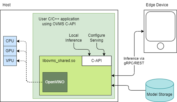
OpenVINO Model Server is typically started as a separate process or run in a container where the client application communicates over a network connection. Now, as you can see above, it is possible to link the model server as a shared library inside the client application and use the internal C API to execute internal inference methods.

We demonstrate the concept in a simple example below and show the impact on latency.

‍

Example C-API Usage

NOTE: complete end to end inference demonstration via C-API with example app can be found here: https://docs.openvino.ai/latest/ovms_demo_capi_inference_demo.html  

To start using the Model Server C-API, we need to prepare a model and configuration file. Download an example dummy model from our GitHub repo and prepare a config.json file to serve this model. “Dummy” model adds value 1 to all numbers inside an input.

‍

Download Model

wget https://github.com/openvinotoolkit/model_server/raw/main/src/test/dummy/1/dummy.{xml,bin} -P models/dummy/1

‍

Create Config File

{ 
    "model_config_list": [ 
        {"config": { 
                "name": "dummy", 
                "base_path": "./models/dummy"}} 
    ] 
} 

‍

Get libovms_shared.so

Next, download and unpack the OVMS library. The library can be obtained from GitHub release page. There are 2 packages – one for Ubuntu 20 and one for RedHat 8.7. There is also documentation showing how to build the library from source. For purpose of this demo, we will use the Ubuntu version:

wget https://github.com/openvinotoolkit/model_server/releases/download/v2022.3/ovms_ubuntu.tar.gz && tar -xvf ovms_ubuntu.tar.gz

‍

Start Server

To start the server, use ServerStartFromConfigurationFile. There are many options, all of which are documented in the header file. Let’s launch the server with configuration file and optional log level error:

OVMS_ServerSettings* serverSettings; 
OVMS_ModelsSettings* modelsSettings; 
OVMS_Server* srv; 
OVMS_ServerSettingsNew(&serverSettings); 
OVMS_ModelsSettingsNew(&modelsSettings); 
OVMS_ServerNew(&srv); 
OVMS_ServerSettingsSetLogLevel(serverSettings, OVMS_LOG_ERROR);  // Make the serving silent 
OVMS_ModelsSettingsSetConfigPath(modelsSettings, "./config.json");  // Previously created file 
OVMS_ServerStartFromConfigurationFile(srv, serverSettings, modelsSettings);  // Start the server 

‍

Input Data Preparation

Use OVMS_InferenceRequestInputSetData call, to provide input data with no additional copy operation. In InferenceRequestNew call, we can specify model name (the same as defined in config.json) and specific version (or 0 to use default). We also need to pass input names, data precision and shape information. In the example we provide 10 subsequent floating-point numbers, starting from 0.

const char* MODEL_NAME = "dummy"; 
const uint64_t MODEL_VERSION = 1; 
const char* INPUT_NAME = "b"; 
constexpr size_t NUM_OF_ELEMENTS = 10; 
constexpr std::array SHAPE = {1, NUM_OF_ELEMENTS}; 
OVMS_InferenceRequest* request; 
OVMS_InferenceRequestNew(&request, srv, MODEL_NAME, MODEL_VERSION); 
OVMS_InferenceRequestAddInput(request, INPUT_NAME, OVMS_DATATYPE_FP32, SHAPE.data(), SHAPE.size()); 
std::array data{0, 1, 2, 3, 4, 5, 6, 7, 8, 9}; 
OVMS_InferenceRequestInputSetData(request, INPUT_NAME, data.data(), sizeof(data), OVMS_BUFFERTYPE_CPU, 0); 

‍

Invoke Synchronous Inference

Simply call OVMS_Inference. This is required to pass response pointer and receive results in the next steps.

OVMS_InferenceResponse* response; 
OVMS_Inference(srv, request, &response); 

‍

Read Results

Use call OVMS_InferenceResponseGetOutput API call to read the results. There are bunch of metadata we can read optionally, such as: precision, shape, buffer type and device ID. The expected output after addition should be:

1, 2, 3, 4, 5, 6, 7, 8, 9, 10,

const char* outputName; 
OVMS_DataType dataType; 
const uint64_t* shape; 
uint32_t dimCount; 
const void* outputData; 
size_t byteSize; 
OVMS_BufferType bufferType; 
uint32_t deviceId; 
OVMS_InferenceResponseGetOutput(response, 0, 
        &outputName, &dataType, &shape, &dimCount, &outputData, &byteSize, &bufferType, &deviceId); 
for (int i = 0; i < NUM_OF_ELEMENTS; i++) 
std::cout << ((float*)outputData)[i] << ", "; 
std::cout << std::endl;

‍

Check the header file to learn more about the supported methods and their parameters.

‍

Compile and Run Application

In this example we omitted error handling and resource cleanup upon failure. Please refer to the full demo instructions for a more complete example.

‍

Performance Analysis

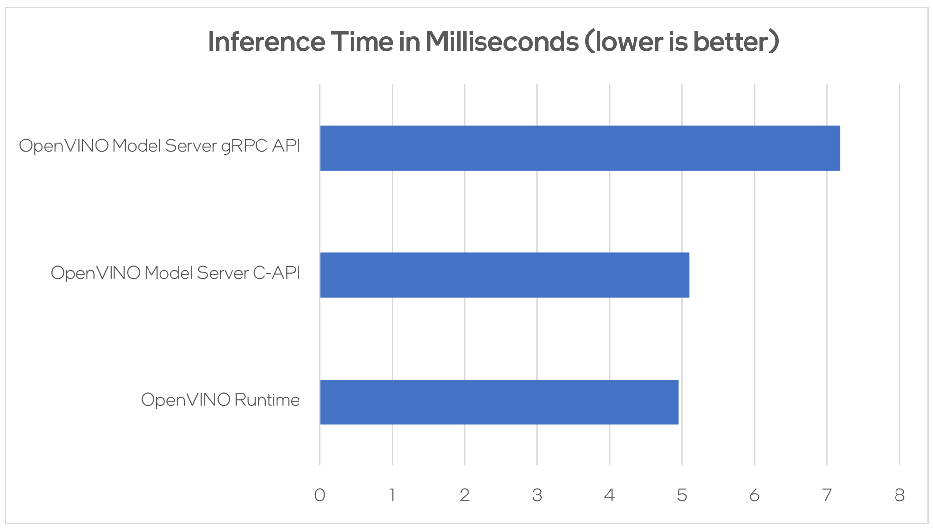
Using benchmarking tools from OpenVINO Runtime and both the C-API and gRPC API in OpenVINO Model Server, we can compare inference results via C-API to typical scenario of gRPC or direct integration of OpenVINO Runtime. The Resnet-50-tf model from Open Model Zoo was used for the testing below.

‍

Hardware configuration used:

- 1-node, Intel Xeon Gold 6252 @ 2.10GHz processor with 256GB (8 slots/16GB/2666) total DDR memory, HT on, Turbo on, Ubuntu 20.04.2 LTS,5.4.0-109-generic kernel

- Intel S2600WFT motherboard

Tested by Intel on 01/31/2023.

‍

Conclusion

With the new method of embedding OVMS into C++ applications, users can decrease inference latency even further by entirely skipping the networking part of model serving. The C-API is still in preview and has some limitations, but in its current state is ready to integrate into C++ applications. If you have questions or feedback, please file an issue on GitHub.

Read more:

• Complete API description: https://docs.openvino.ai/latest/ovms_docs_c_api.html  
• End to end demo: https://docs.openvino.ai/latest/ovms_demo_capi_inference_demo.html  

‍

In this blog you will learn how to set up horizontal autoscaling in Kubernetes using inference performance metrics exposed by OpenVINO™ Model Server. This will enable efficient scaling of model serving pods for inference on Intel® CPUs and GPUs.

Why use custom metrics?

OpenVINO™ Model Server provides high performance AI inference on Intel CPUs and GPUs that can be scaled in Kubernetes. However, when it comes to automatic scaling in Kubernetes, the Horizontal Pod Autoscaler by default, relies on CPU utilization and memory usage metrics only. Although resource consumption indicates how busy the application is, it does not clearly say whether serving provides expected quality of service to the clients or not. Since OpenVINO Model Server exposes performance metrics, we can automatically scale based on service quality rather than resource utilization.

The first metric that comes to mind when thinking about service performance is the duration of request processing, otherwise known as latency. For example, mean or median over a specified period or latency percentiles. OpenVINO Model Server provides such metrics but setting autoscaling based on latency requires specific knowledge about each model and the environment where the inference is running in order to properly set thresholds that trigger scaling.

While autoscaling based on latency works and may be a good choice when you have model-specific knowledge, we will instead focus on a more generic metric using ovms_requests_streams_ratio. Let’s dive into what this means.

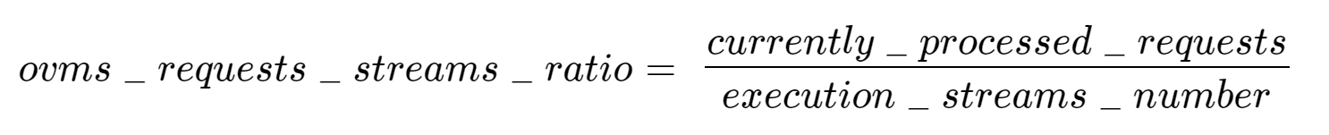
In the equation above:

• currently_processed_requests - number of inference requests to a model being processed by the service at a given time.

• execution_streams_number – number of execution streams. (When a model is loaded on the device, its computing units are divided into streams. Each stream independently handles inference requests, meaning that the number of streams defines how many inferences can be run on the device in parallel. Note that the more streams there are, the less powerful they are, so we get more throughput at a cost of higher minimal latency / inference time.)

‍

In this equation, for any model exceeding a value of 1 indicates that requests are starting to queue up. Setting the autoscaler threshold for the ovms_requests_streams_ratio metric is somewhat of an arbitrary decision that should be made by a cluster administrator. Setting the threshold too low will result in underutilization of nodes and setting it too high will force the system to work with insufficient resources for extended periods of time. Now that we have chosen a metric for autoscaling, let’s start setting it up.

Deploy Model Server with Autoscaling Metrics

First, we need to create a deployment of OpenVINO Model Server in Kubernetes. To do this, follow instructions to install the OpenVINO Operator in your Kubernetes cluster. Then create a configuration where we can specify the model to be served and enable metrics:

apiVersion: v1 
kind: ConfigMap 
metadata: 
  name: ovms-config 
  namespace: default 
data: 
  ovms_config.json: | 
    { 
    "model_config_list": [ 
         { 
            "config": { 
                 "name": "resnet50-int8", 
                 "base_path": "gs://ovms-public-eu/resnet50-binary" 
            } 
         } 
     ], 
     "monitoring": 
         { 
             "metrics": 
             { 
                 "enable": true 
             } 
         } 
    }

‍

Create ConfigMap:

kubectl apply -f https://raw.githubusercontent.com/openvinotoolkit/operator/main/examples/hpa_custom_metrics/ovms_config.yaml

‍

With the configuration in place, we can deploy OpenVINO Model Server instance:

apiVersion: intel.com/v1alpha1 
kind: ModelServer 
metadata: 
  name: demo 
spec: 
  image_name: 'openvino/model_server:2022.2' 
  service_parameters: 
    grpc_port: 8080 
    rest_port: 8081 
  models_settings: 
    single_model_mode: false 
    config_configmap_name: 'ovms-config' 
    config_path: '/config/ovms_config.json' 
  server_settings: 
    file_system_poll_wait_seconds: 0 
    log_level: INFO 
  deployment_parameters: 
    replicas: 1

‍

Create ModelServer resource:

kubectl apply -f https://raw.githubusercontent.com/openvinotoolkit/operator/main/examples/hpa_custom_metrics/ovms.yaml

Deploy and Configure Prometheus

Next, we need to read serving metrics and expose them to the Horizontal Pod Autoscaler. To do this we will deploy Prometheus to collect serving metrics and the Prometheus Adapter to expose them to the autoscaler.  

Deploy Prometheus Monitoring Tool

Let’s start with Prometheus. In the example below we deploy a simple Prometheus instance via the Prometheus Operator. To deploy the Prometheus Operator, run the following command:

kubectl create -f https://raw.githubusercontent.com/prometheus-operator/prometheus-operator/v0.59.2/bundle.yaml

Next, we need to configure role-based access control to give Prometheus permission to access the Kubernetes API:

kubectl apply -f https://raw.githubusercontent.com/openvinotoolkit/operator/main/examples/hpa_custom_metrics/prometheus_rbac.yaml

The last step is to create a Prometheus instance by deploying Prometheus resource:

kubectl apply -f https://raw.githubusercontent.com/openvinotoolkit/operator/main/examples/hpa_custom_metrics/prometheus.yaml 

If the deployment was successful, a Prometheus service should be running on port 9090. You can set up a port forward for this service, enabling access to the web interface via localhost on your machine:

kubectl port-forward svc/prometheus-operated 9090:9090

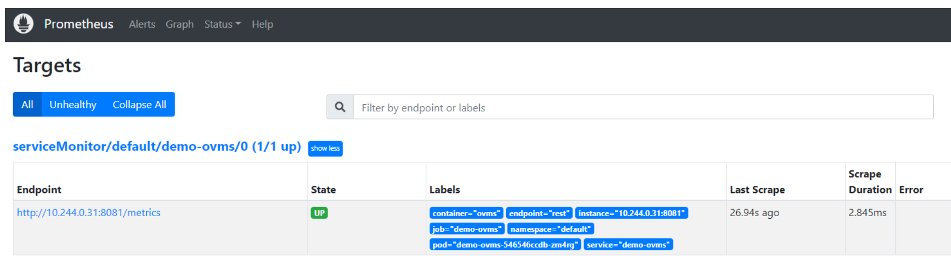
Now, when you open http://localhost:9090 in a browser you should see the Prometheus user interface. Next, we need to expose the Model Server to Prometheus by creating a ServiceMonitor resource:

kubectl apply -f https://raw.githubusercontent.com/openvinotoolkit/operator/main/examples/hpa_custom_metrics/service_monitor.yaml

Once it’s ready, you should see a demo-ovms target in the Prometheus UI:

‍

Now that the metrics are available via Prometheus, we need to expose them to the Horizonal Pod Autoscaler. To do this, we deploy the Prometheus Adapter.

‍

Deploy Prometheus Adapter

Prometheus Adapter can be quickly installed via helm or step-by-step via kubectl. For the sake of simplicity, we will use helm3. Before deploying the adapter, we will prepare a configuration that tells it how to expose the ovms_requests_streams_ratio metric:  

apiVersion: v1 
kind: ConfigMap 
metadata: 
  name: adapter-config 
  namespace: default 
data: 
  config.yaml: |+ 
    rules: 
    - seriesQuery: 'ovms_current_requests' 
      resources: 
        overrides: 
          namespace: 
            resource: namespace 
          pod: 
            resource: pod 
      name: 
        matches: "ovms_current_requests" 
        as: "ovms_requests_streams_ratio" 
      metricsQuery: avg(avg_over_time(ovms_current_requests{<<.LabelMatchers>>}[1m]) 
 / avg_over_time(ovms_streams{<<.LabelMatchers>>}[1m])) by (<<.GroupBy>>)

Create a ConfigMap:

kubectl apply –f https://raw.githubusercontent.com/openvinotoolkit/operator/main/examples/hpa_custom_metrics/prometheus_adapter_config.yaml

Now that we have a configuration, we can install the adapter:

helm repo add prometheus-community https://prometheus-community.github.io/helm-charts

helm repo update 

helm install --set 'prometheus.url=http://prometheus-operated.default.svc' --set 'rules.existing=adapter-config' prometheus-adapter prometheus-community/prometheus-adapter

‍

Keep checking until custom metrics are available from the API:

kubectl get --raw /apis/custom.metrics.k8s.io/v1beta1 | jq 
{ 
  "kind": "APIResourceList", 
  "apiVersion": "v1", 
  "groupVersion": "custom.metrics.k8s.io/v1beta1", 
  "resources": [ 
    { 
      "name": "namespaces/ovms_requests_streams_ratio", 
      "singularName": "", 
      "namespaced": false, 
      "kind": "MetricValueList", 
      "verbs": [ 
        "get" 
      ] 
    }, 
    { 
      "name": "pods/ovms_requests_streams_ratio", 
      "singularName": "", 
      "namespaced": true, 
      "kind": "MetricValueList", 
      "verbs": [ 
        "get" 
      ] 
    } 
  ] 
}

Once you see the output above, you can configure the Horizontal Pod Autoscaler to use these metrics.

‍

Set up Horizontal Pod Autoscaler

As mentioned previously, we will set up autoscaling based on the ovms_requests_streams_ratio metric and target an average value of 1. This will try to keep all streams busy all the time while preventing requests from queueing up. We will set minimum and maximum number of replicas to 1 and 3, respectively, and the stabilization window for both upscaling and downscaling to 120 seconds:

kind: HorizontalPodAutoscaler 
apiVersion: autoscaling/v2 
metadata: 
  name: ovms-hpa 
spec: 
  scaleTargetRef: 
    apiVersion: intel.com/v1alpha1 
    kind: ModelServer 
    name: demo 
  minReplicas: 1 
  maxReplicas: 3 
  metrics: 
  - type: Pods 
    pods: 
      metric: 
        name: ovms_requests_streams_ratio 
      target: 
        type: AverageValue 
        averageValue: 1 
  behavior: 
    scaleDown: 
      stabilizationWindowSeconds: 120 
    scaleUp: 
      stabilizationWindowSeconds: 120

Create HorizontalPodAutoscaler:

kubectl apply -f https://raw.githubusercontent.com/openvinotoolkit/operator/main/examples/hpa_custom_metrics/ovms_hpa.yaml 

Once deployed, you can generate some load for your model and see the results. Below you can see how Horizontal Pod Autoscaler scales the number of replicas by checking its status:

kubectl describe hpa ovms-hpa

This data can also be visualized with a Grafana dashboard:

‍

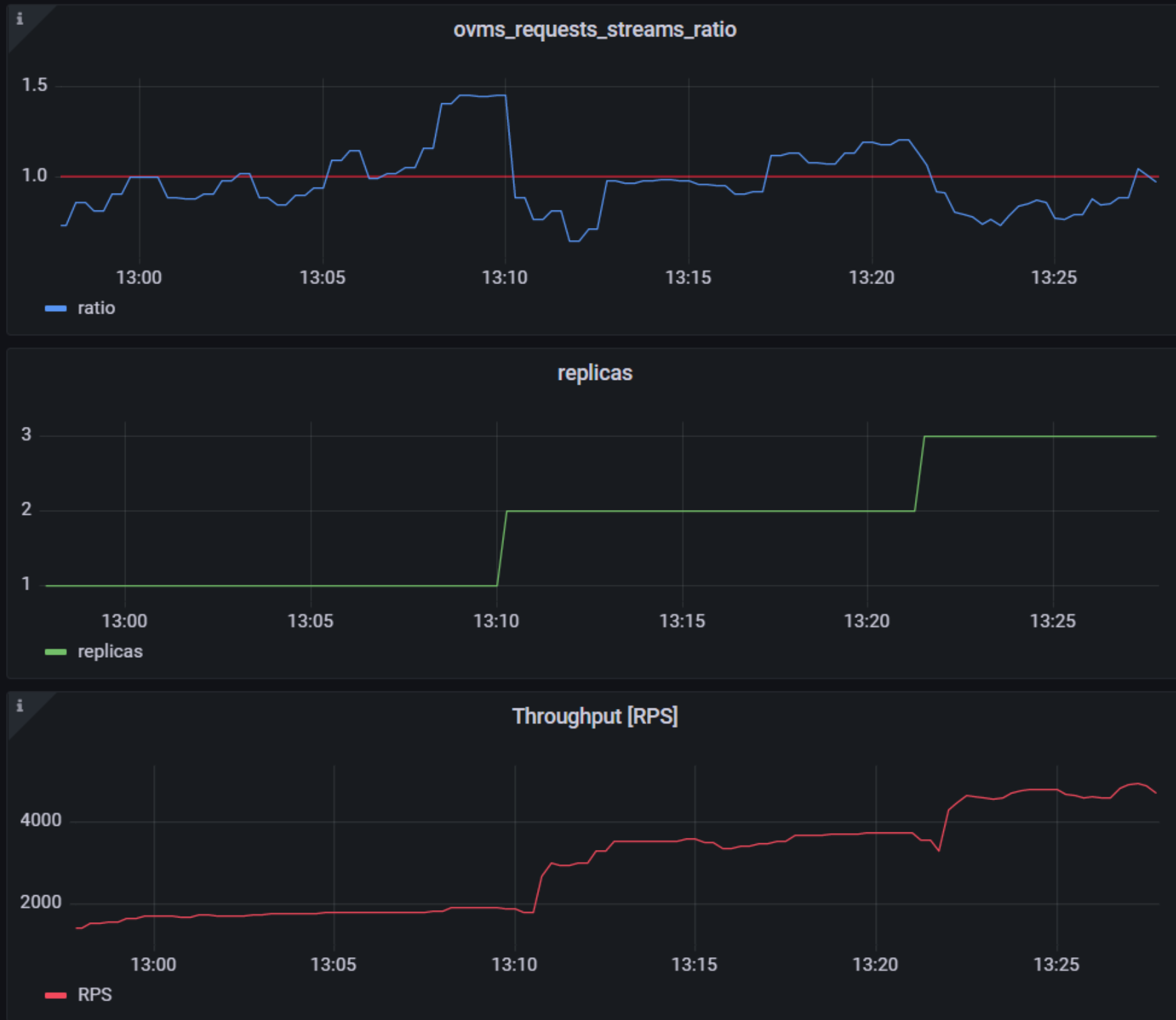
As you can see, with OpenVINO Model Server metrics, you can quickly set up inferencing system with monitoring and autoscaling for any model. Moreover, with custom metrics, you can set up autoscaling for inference on any Intel CPUs and GPUs.  

See also:

• Load Balancing OpenVINO Model Server Deployments with Red Hat‍
• Kubernetes Device Plugin for Intel GPU‍
• OpenVINO Model Server metrics

‍

Introduction

CPU plugin of OpenVINO™ toolkit as one of the most important part, which is powered by oneAPI Deep Neural Network Library (oneDNN) can help user achieve high performance inference of neural networks on Intel®x86-64 CPUs. The CPU plugin detects the Instruction Set Architecture (ISA) in the runtime and uses Just-in-Time (JIT) code generation to deploy the implementation optimized for the latest supported ISA.

In this blog, you will learn how layer primitives been optimized by implementation of ISA extensions and how to change the ISA extensions’ optimized kernel function at runtime for performance tuning and debugging.

After reading this blog, you will start to be proficient in AI workloads performance tuning and OpenVINO™ profiling on Intel® CPU architecture.

CPU Profiling

OpenVINO™ provide Application Program Interface (API) which is easy to turn on CPU profiling and analyze performance of each layer from the bottom level by executed kernel function. Firstly, enable performance counter profiling with executed device during device property configuration before model compiling with device. Learn detailed information from document of OpenVINO™ Configuring Devices.

core.set_property("CPU", ov::enable_profiling(true));

Then, you are allowed to get object of profiling info from inference requests which complied with the CPU device plugin.

auto perfCounts = infer_request.get_profiling_info();

Please note that performance profiling information generally can get after model inference. Refer below code implementation and add this part after model inference. You are possible to get status and performance of layer execution. Follow below code implement, you will get performance counter printing in order of the execution time from largest to smallest.

bool sort_pc_descend(const ov::ProfilingInfo& profiling1, const ov::ProfilingInfo& profiling2) {
    return profiling1.real_time > profiling2.real_time;
}
...
int tmain(int argc, tchar* argv[]) {
	...
	//objects init
	int layersize = 0;
	bool sort_pc_descend = 1;
	std::chrono::microseconds total = std::chrono::microseconds::zero();
	std::chrono::microseconds total_cpu = std::chrono::microseconds::zero();
	static const char* status_names[] = {"NOT_RUN", "OPTIMIZED_OUT", "EXECUTED"};

	//print row of title
	std::cout << "layerName\t"
	    << "execStatus\t"
	    << "layerType:"
	    << "execType\t";
	std::cout << "realTime (ms)\t"
	    << "cpuTime (ms)\t"
	    << " proportion(%)" << std::endl;

	//calculate executed layers total latency
	for (const auto& layer : perfCounts) {
	    if (std::string(status_names[(int)layer.status]).compare("EXECUTED") == 0) {
	        total += layer.real_time;
	        total_cpu += layer.cpu_time;
	    }
	}

	//print executed layer name, status, execution kernel funtion, CPU execution time and percentage of total model latency
	std::sort(perfCounts.begin(), perfCounts.end(), sort_pc_descend);
	for (const auto& layer : perfCounts) {
	    if (std::string(status_names[(int)layer.status]).compare("EXECUTED") == 0) {
	        std::cout << layer.node_name << "\t";
	        std::cout << ((int)layer.status < (sizeof(status_names) / sizeof(status_names[0]))
	                    ? status_names[(int)layer.status]
	                    : "INVALID_STATUS") << "\t";
	        std::cout << layer.node_type << ":" << layer.exec_type << "\t";
	        std::cout << std::to_string(layer.real_time.count() / 1000.0) << "\t"
	            << std::to_string(layer.cpu_time.count() / 1000.0) << "\t";
	        std::cout << (layer.real_time * 1.0 / total) * 100 << std::endl;
	        layersize += 1;
	    }
	}
}

CPU Dispatching

By enabling device profiling and printing exec_type of layers, you will get the specific kernel functions which powered by oneDNN during runtime execution. Use TensorFlow* ResNet 50 INT8 model for execution and pick the first 10 hotspot layers on 4th Gen Intel® Xeon Scalable processor (code named Sapphire Rapids) as an example:

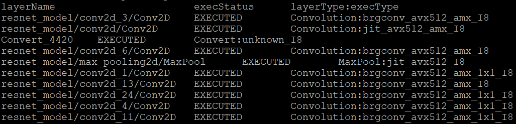
From execution type of layers, it would be helpful to check which oneDNN kernel function used, and the actual precision of layer execution and the optimization from supported ISA on this platform.

Normally, oneDNN is able to detect to certain ISA, and OpenVINO™ allow to use latest ISA with higher priority. If you want to compare optimization rate between different ISA, can use the ONEDNN_MAX_CPU_ISA environment variable to limit processor features with older instruction sets. Follow this link to check oneDNN supported ISA.

Please note, Intel® Advanced Matrix Extensions (Intel® AMX) ISA start to be supported since 4th Gen Intel® Xeon Scalable processor. You can refer Intel® Product Specifications to check the supported instruction set of your current platform.

The ISAs are partially ordered:

·      SSE41 < AVX < AVX2 < AVX2_VNNI <AVX2_VNNI_2,

·      AVX2 < AVX512_CORE < AVX512_CORE_VNNI< AVX512_CORE_BF16 < AVX512_CORE_FP16 < AVX512_CORE_AMX <AVX512_CORE_AMX_FP16,

·      AVX2_VNNI < AVX512_CORE_FP16.

To use CPU dispatcher control, just set the value of ONEDNN_MAX_CPU_ISA environment variable before executable program which contains the OpenVINO™ device profiling printing, you can use benchmark_app as an example:

ONEDNN_MAX_CPU_ISA=AVX512_CORE_VNNI benchmark_app -m ~/models/public/resnet-50-tf/FP32-INT8/resnet-50-tf.xml -d CPU -pcsort sort

The benchmark_app provides the option which named “-pcsort” can report performance counters and order analysis information by order of layers execution time when set value of the option by “sort”.

In this case, we use above code implementation can achieve similar functionality of benchmark_app “-pcsort” option. User can consider try to add the code implementation into your own OpenVINO™ program like below:

ONEDNN_MAX_CPU_ISA=AVX512_CORE_VNNI ./classification_profiling ~/models/public/resnet-50-tf/FP32-INT8/resnet-50-tf.xml ./sample_640×426.bmp CPU

After setting the CPU dispatcher, the kernel execution function has been switched from AVX512_CORE_AMX to AVX512_CORE_VNNI. Then, the performance counters information would be like below:

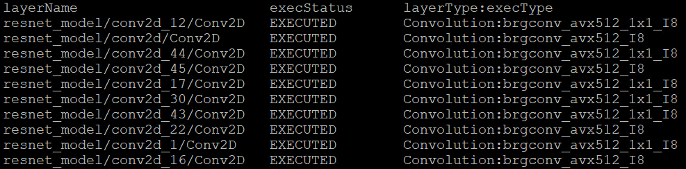
You can easily find the hotspot layers of the same model would be changed when executed by difference kernel function which optimized by implementation of different ISA extensions. That is also the optimization differences between architecture platforms.

Tuning Tips

Users can refer the CPU dispatcher control and OpenVINO™ device profiling API to realize performance tuning of your inference program between CPU architectures. It will also be helpful to developer finding out the place where has the potential space of performance improvement.

For example, the hotspot layer generally should be compute-intensive operations like matrix-matrix multiplication; General vector operations which is not target to artificial intelligence (AI) / machine learning (ML) workloads cannot be optimized by Intel® AMX and Intel® Deep Learning Boost (Intel® DL Boost), and the memory accessing operations, like Transpose which maybe cannot parallelly optimized with instruction sets. If your inference model remains large memory accessing operations rather than compute-intensive operations, you probably need to be focusing on RAM bandwidth optimization.

‍