.png)
Kunda
Xu
OpenVINO optimizer Latent Diffusion Models (LDM) for super-resolution
OpenVINO optimizer Latent Diffusion Models(LDM) for super-resolution
Introduction
A computer vision approach called image super-resolution aims to increase the resolution of low-resolution images so that they are clearer and more detailed. Applicationsfor super-resolution include the processing of medical images, surveillancefootage, and satellite images.
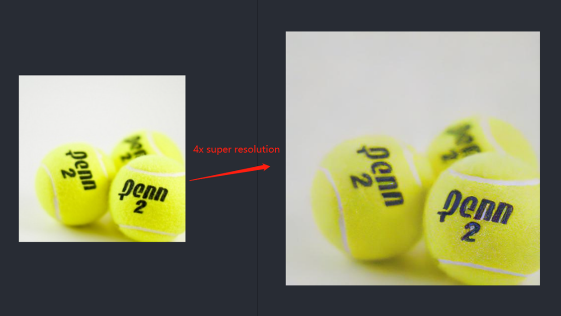
The LDM (LatentDiffusion Models) Super Resolution model, a deep learning-based approach to photo super-resolution, was developed by the Hugging Face Research team. The residual network (ResNet) architecture, a type of convolutional neural network(CNN) created to address the issue of vanishing gradients in deep neuralnetworks.
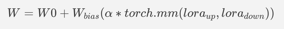
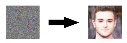
Diffusion models are generative models,meaning that they are used to generate data similar to the data on which they are trained. Fundamentally, Diffusion Models work by destroying training data through the successive addition of Gaussian noise, andthen learning to recover the data by reversing this noising process. After training, we can use the Diffusion Model to generatedata by simply passing randomly sampled noise through the learned denoising process.
Diffusion Model is a latent variable model which maps to the latent space using a fixed Markov chain. This chain gradually adds noise to thedata in order to obtain the approximate posterior.
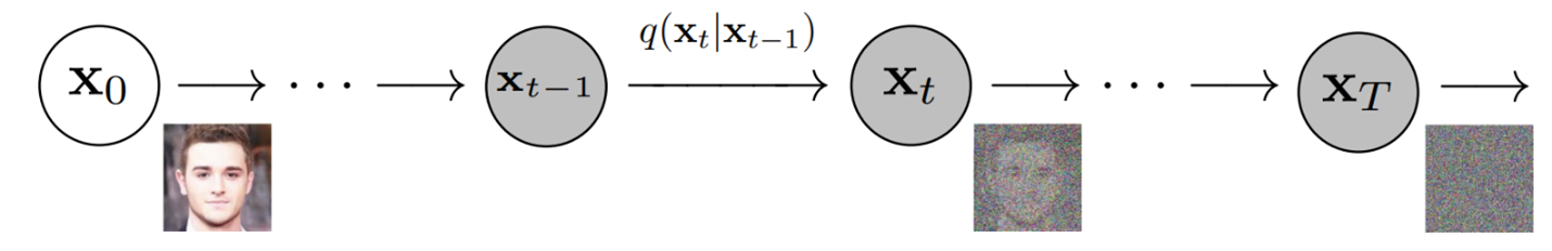
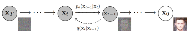
Ultimately, the image is asymptotically transformed to pure Gaussian noise. The goal of training a diffusion model is to learn the reverse process. By traversing backward along this chain, we can generate new data.
Requirement
- Optimum-intel Optimum Intel is the interface betweenthe HuggingFace Transformers and Diffusers libraries and the differenttools and libraries provided by Intel to accelerate end-to-end pipelines onIntel architectures.
Intel Neural Compressor is an open-source library enabling the usageof the most popular compression techniques such as quantization, pruning and knowledge distillation
- OpenVINO™ is an open-sourcetoolkit for optimizing and deploying AI inference which can boost deep learningperformance in computer vision, automatic speech recognition, natural language processing and other common task.
- optimum-intel==1.5.2(include openvino)
- openvino
- openvino-dev
- diffusers
- pytorch >= 1.9.1
- onnx >= 1.13.0
Reference: optimum-intel-ldm-super-resolution-4x
QuickStart Demo
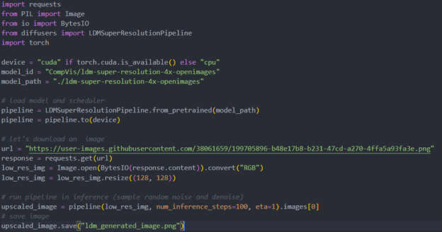
Original repo is from HuggingFace CompVis/ldm-super-resolution-4x-openimages,we are reference to build our pipeline to implement super-resolution related function.
To transformand acceleration optimize the pipeline by openvino, there are 3 steps need to do.
- Step1. Install the requirement package and initial environment.
- Step2. Convert original model to openvino IR model.
- Step3. Build OpenVINO super resolution pipeline.
Now, Let’s start with the content of our tutorial.
Step 1. Install the requirementpackage and initial environment
OpenVINO has the standard installation process, we can directly refer tothe official OpenVINO documentation to install.
Reference: Install OpenVINO by source code for Linux
Reference: Install OpenVINO by release package
Optimum Intel also can refer the standard guide.
Reference: Optimum-intel install guide
(Optional) Install the latest stable release by pipe :
# pip install openvino, openvino-dev
# pip install"optimum[openvino,nncf]"
Step 2. Convert originalmodel to OpenVINO IR model
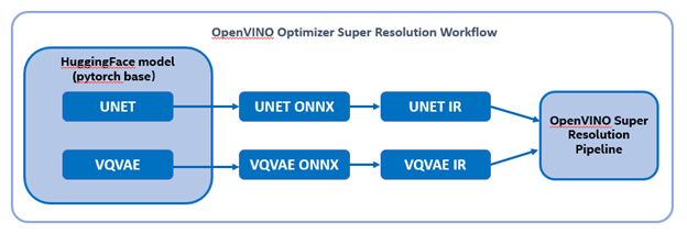
Firstly, run pipe the HuggingFace pipeline, it will automate download the models, and we need to convert them from pytorch->onnx->IR, to enable the model by OpenVINO.
%20workflow.png)
The LDM (LatentDiffusion Models) Super Resolution model has two part of sub-models: unet and vqvae,we should convert each of them in to IR model.
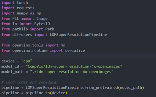
The reference source code for model convert,also we provide the script in the GitHub repo : ov-ldm4x-model-convert.py
Initial parameter and the ov-pipeline
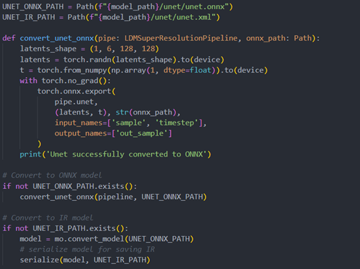
Unet sub-model convert to IR
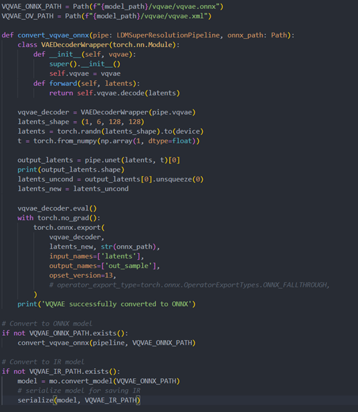
Vqvae sub-model convert to IR
Step 3. Build OpenVINOsuper resolution pipeline
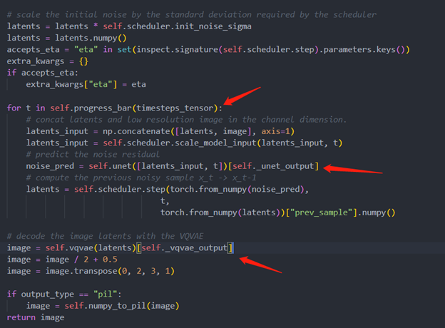
The LDM (Latent Diffusion Models) Super Resolution OpenVINO pipeline main function part code, the whole pipeline script is provided in GitHub repo: ov-ldm4x-pipeline.py
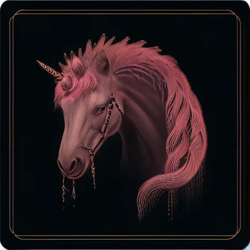
Inference Result