

OpenVINO Blog

Q2'22: Technology update – low precision and model optimization
Authors
Alexander Kozlov, Alexander Suslov, Pablo Munoz, Vui Seng Chua, Nikolay Lyalyushkin, Yury Gorbachev, Nilesh Jain
Summary
This quarter we observed an increased interest in pruning methods for Transformer-based architectures (BERT, etc.). The main reason for that, as we see it, is a huge success of this architecture in many domains such as NLP, Computer Vision, Speech and Audio processing. NAS methods continue beating handcrafted models on various tasks and benchmarks. As usual, DL model optimization is still a huge area with lots of people involved both from academia and industry.
Papers with notable results
Quantization
- Differentiable Model Compression via Pseudo Quantization Noise by Facebook AI Research (https://arxiv.org/pdf/2104.09987v1.pdf).In this paper, authors propose a DIFFQ method that uses a pseudo quantization noise to approximate quantization at train time, as a differentiable alternative to STE, both with respect to the unquantized weights and number of bits used. With a single penalty level λ, DIFFQ optimizes the number of bits per weight or group of weights to achieve a given trade-off between model size and accuracy. The method outperforms a regular QAT method at a low-bit quantization on different tasks.
- Do All MobileNets Quantize Poorly? Gaining Insights into the Effect of Quantization on Depthwise Separable Convolutional Networks Through the Eyes of Multi-scale Distributional Dynamics by Waterloo Artificial Intelligence Institute (https://arxiv.org/pdf/2104.11849v1.pdf).Authors investigate the impact of quantization on the weight and activation distributional dynamics as information propagates from layer to layer, as well as overall changes in distributional dynamics at the network level. This fine-grained analysis revealed significant dynamic range fluctuations and a “distributional mismatch” between channel wise and layer wise distributions in depth-wise CNNs such as MobileNet that lead to increasing quantized degradation and distributional shift during information propagation. Furthermore, analysis of the activation quantization errors shows that there is greater quantization error accumulation in depth-wise CNNs compared to regular CNNs.
- TENT: Efficient Quantization of Neural Networks on the tiny Edge with Tapered Fixed Point by Neuromorphic AI Lab, University of Texas (https://arxiv.org/pdf/2104.02233v1.pdf).An interesting read for those who are not aware of taper and posit numerical formats. Authors propose a tapered fixed-point quantization algorithm that adapts the numerical format to best represent the layer wise dynamic range and distribution of parameters within a Tiny ML model. They do not provide extensive results but show a superior performance vs. Vanilla fixed-point quantization.
- n-hot: Efficient Bit-Level Sparsity for Powers-of-Two Neural Network Quantization by Sony (https://arxiv.org/pdf/2103.11704v1.pdf).One more method for power-of-two quantization as an alternative to APoT method which also allows reducing the model size. The method uses bit-level sparsity and introduces subtraction of PoT terms. It also applies two-stage long fine-tuning during quantization. This helps to achieve superior results vs. vanilla PoT and APoT methods.
- Network Quantization with Element-wise Gradient Scaling by Yonsei University (https://arxiv.org/pdf/2104.00903v1.pdf).This paper proposes an element-wise gradient scaling (EWGS), a simple alternative to the STE, training a quantized network better than the STE in terms of stability and accuracy. Given a gradient of the discretizer output, EWGS adaptively scales up or down each gradient element, and uses the scaled gradient as the one for the discretizer input to train quantized networks via backpropagation. The method achieves very promising results on CIFAR and ImageNet dataset in low-bit quantization setup (1-2 bits).
- Q-ASR: Integer-only Zero-shot Quantization for Efficient Speech Recognition by Berkeley (https://arxiv.org/pdf/2103.16827v1.pdf).The paper about data-free quantization of the automatic speech recognition models. As usual, the authors use statistics from BatchNorm layers and backpropagation to construct a synthetic dataset. They achieve good results for QuartzNet and JasperDR model that contains BatchNorm.
- Neuro evolution-Enhanced Multi-Objective Optimization for Mixed-Precision Quantization by Intel Labs (https://arxiv.org/pdf/2106.07611v1.pdf).In this paper, authors present a framework for automated mixed-precision quantization that optimizes multiple objectives. The framework relies on Neuro evolution-Enhanced Multi-Objective Optimization (NEMO) to find Pareto optimal mixed-precision configurations for memory and bit-operations objectives. Authors also apply some tricks on top of NEMO to improve the goodness of the Pareto frontier. The method shows state-of-the-art results on several ImageNet models.
- Post-Training Sparsity-Aware Quantization by Israel Institute of Technology(https://arxiv.org/pdf/2105.11010v1.pdf).In this paper, authors propose a complicated quantization scheme that can be done post-training and leverages multiple assumptions, like bit-sparsity of weights and activations, bell-shaped distribution, many zeros in activations. Essentially, the proposed scheme picks the most significant n bits from the 8-bit value representation, while skipping leading zero-value bits. Authors also make projections on the area that requires to implement inference of such quantized models, namely for sysytolic-based architectures and Tensor Cores. They claim SOTA results, for example, for ResNet-50 on ImageNet: -0.18% relative degradation in accuracy, 2× speedup over conventional SA, and an additional 22% SA area overhead. Code is available at https://github.com/gilshm/sparq.
- On the Distribution, Sparsity, and Inference-time Quantization of Attention Values in Transformers by Stony Brook University (https://arxiv.org/pdf/2106.01335v1.pdf).A study about quantization of Transformer-based models (BERT-like). Authors focus on reducing number of bits required to represent information of attentions masks in Self-Attention block. They claim that in many cases it is possible to prune and quantize the mask (to lower bits using non-uniform quantization). The code for the analysis and data are available at https://github.com/StonyBrookNLP/spiqa.
Sparsity
- Accelerated Sparse Neural Training: A Provable and Efficient Method to Find N:M Transposable Masks by Habana and Labs (https://arxiv.org/pdf/2102.08124.pdf). The paper proposed a method to accelerate training using N:M weight sparsity with transposable-fine-grained sparsity mask where the same mask can be used for both forward and backward passes. This mask ensures that both the weight matrix and its transpose follow the same sparsity pattern; thus the matrix multiplication required for passing the error backward can also be accelerated. Experiments show 2x speed-up with no accuracy degradation over vision and language models.
- Post-training deep neural network pruning via layer-wise calibration by Intel (https://arxiv.org/abs/2104.15023v1). The paper introduces a method for accurate unstructured model pruning in the post-training scenario. The method is based on a layer-wise tuning (knowledge distillation) approach when the knowledge from the original model is distilled to the optimizing counterpart in a layer-wise fashion. Authors also propose a way of data-free accurate pruning. The method is available here.
- Carrying out CNN Channel Pruning in a White Box by Tencent and China universities (https://arxiv.org/pdf/2104.11883v1.pdf). The paper proposes a method to model the contribution of each channel to differentiating categories. The authors developed a class-wise mask for each channel, implemented in a dynamic training manner w.r.t. the input image’s category. On the basis of the learned class-wise mask, they perform a global voting mechanism to remove channels with less category discrimination. The method shows comparable results vs. other Filter Pruning criterions but it performance is worse than RL or evolutionary-based method, e.g. LeGR.
- Rethinking Network Pruning— under the Pre-train and Fine-tune Paradigm by Moffett AI (https://arxiv.org/pdf/2104.08682v1.pdf).The paper proposes a method for sparse pruning Transformer-based models. The method exploits the magnitude-based criterium to prune unimportant weights and uses knowledge distillation supervision from the original fine-tuned model. The knowledge distillation is based on MSE loss and connects multiple layers from the original model with the same layers in the pruning counterpart. The method shows good results on the tasks from GLUE benchmark: 95% of weights are pruned while preserving accuracy on most of the tasks.
- MLPruning: A Multilevel Structured Pruning Framework for Transformer-based Models by Berkeley University (https://arxiv.org/pdf/2105.14636v1.pdf). A method to optimize Transformer-based architectures (BERT) that consists of three different levels of structured pruning: 1) Head pruning for multi-head attention; 2) Row pruning for general fully-connected layers; and 3) block-wise sparsity pruning for all weight matrices. To benefit from block sparsity, authors use block-sparse MatMul kernel from Triton SW. They achieve good results on QQP/MNLI/SQuAD, with up to ~3.69xspeedup. Code is available here.
Filter Pruning
- EZCrop: Energy-Zoned Channels for Robust Output Pruning by University of Hong Kong (https://arxiv.org/pdf/2105.03679v2.pdf).The paper introduces a method to interpret channel importance metric in the spatial domain as an energy perspective in the frequency domain. It proposes a computationally efficient FFT-based metric for channel importance. The method slightly outperforms the accuracy of some recent state-of-the-art methods but more computationally efficient at the same time.
- Visual Transformer Pruning by Huawei (https://arxiv.org/pdf/2104.08500v2.pdf).The paper provides a method that identifies the impacts of channels in each layer and then executes pruning accordingly. By encouraging channel-wise sparsity in the Transformer, important channels automatically emerge. A great number of channels with small coefficients can be discarded to achieve a high pruning ratio without significantly compromising accuracy. Authors show that it is possible to prune ~40% of ViT-B/16 model while staying at ~1% of accuracy degradation on ImageNet.
- Convolutional Neural Network Pruning with Structural Redundancy Reduction by The University of Tennessee and 2Sun Yat-sen University (https://arxiv.org/pdf/2104.03438v1.pdf).The paper provides a theoretical analysis of network pruning with statistical modeling from a perspective of redundancy reduction. It also proposes a layer-adaptive channel pruning approach based on structural redundancy reduction which builds a graph for each convolutional layer of a CNN to measure the redundancy existed in each layer (a non-usual approach). The method could prune 55.1% of ResNet-50 FLOPS while staying at ~1% of accuracy drop on ImageNet.
- Model Pruning Based on Quantified Similarity of Feature Maps by University of Science and Technology Beijing (https://arxiv.org/pdf/2105.06052v1.pdf).The paper proposes a new complex criterion to prune filters from any type of convolutional operation. It uses Structural Similarity or Peak Signal to Noise Ratio to find the score of the filters. Despite the fact the paper provides results only on CIFAR dataset, the paper still interesting because it allows pruning filters without fine-tuning while preserving the accuracy. It means that this method can be potentially applied in the post-training scenario to highly redundant models.
- Greedy Layer Pruning: Decreasing Inference Time of Transformer Models by DeepOpinion(https://arxiv.org/pdf/2105.14839v1.pdf).In this paper, authors propose a method to layer pruning (GLP) is introduced to(1) outperform current state of-the-art for layer-wise pruning of Transformer-based architectures without knowledge distillation with long fine-tuning. They focus more on providing an optimization algorithm that requires a modest budget from the resource and price perspective. The method achieves good results on GLUE benchmark and requires only $300 for all 9 tasks.
- Width transfer: on the(in)variance of width optimization by Facebook(https://arxiv.org/pdf/2104.13255.pdf).This work reduces computational overhead in width optimization algorithms(MorphNet, AutoSlim, and DMCP), which in contrast to pruning, improves accuracy by reorganizing width of layers without changing FLOPS. The algorithm uniformly shrinks model's channels and depth, optimizes width on a part of a dataset with smaller images, then the optimized projected network is extrapolated to match original FLOPS and dimensions. Authors can achieve up to 320x overhead reduction without compromising the top-1. Major cons: still the additional cost of width optimization is comparable with initial training time.
Neural Architecture Search
- How Powerful are Performance Predictors in Neural Architecture Search? by Abacus.AI, Bosch and universities(https://arxiv.org/pdf/2104.01177.pdf).The first large-scale study of performance predictors by analyzing 31techniques ranging from learning curve extrapolation, to weight-sharing, supervised learning, “zero-cost” proxies. The code is available at https://github.com/automl/naslib.
- Dynamic-OFA: Runtime DNN Architecture Switching for Performance Scaling on Heterogeneous Embedded Platforms by University of Southampton (https://arxiv.org/pdf/2105.03596v2.pdf). Dynamic-OFA, extends OFA to quickly switch architecture in runtime. Sub-network architectures are sampled from OFA for both CPU and GPU at the offline stage. These architectures have different performance (e.g. latency, accuracy) and are stored in a look-up table to build a dynamic version of OFA without any additional training required. Then, at runtime, Dynamic-OFA selects and switches to optimal sub-network architectures to fit time-varying available hardware resources The approach is up to 3.5x (CPU), 2.4x (GPU) faster for similar ImageNetTop-1 accuracy, or 3.8% (CPU), 5.1% (GPU) higher accuracy at similar latency.
- RHNAS: Realizable Hardware and Neural Architecture Search by Intel Labs (https://arxiv.org/pdf/2106.09180v1.pdf). The paper introduces a NN-HW co-design method that integrates RL-based hardware optimizers with differentiable NAS. It overcomes the challenges associated with sparse validity- a failure point for existing differentiable co-design works. The authors also benchmark RL-based hardware optimizer and use Bayesian hyperparameter optimization to identify the best hyper-parameters for a fair study of a range of standard RL algorithms. The method discovers realizable NN-HW designs with 1.84×lower latency and 1.86× lower energy delay product (EDP) on ImageNet over the default hardware accelerator design.
- NAS-BERT: Task-Agnostic and Adaptive-Size BERT Compression with Neural Architecture Search by MSRA and China universities (https://arxiv.org/pdf/2105.14444v1.pdf). In this paper, authors apply NAS on the pre-training task to search for efficient lightweight NLP models, which can deliver adaptive model sizes given different requirements of memory or latency and apply for different down stream tasks. They also apply block-wise search, progressive shrinking and performance approximation to reduce the search cost and improve the search accuracy. The proposed method demonstrates comparable results on GLUE and SQuAD benchmarks.
- FNAS: Uncertainty-Aware Fast Neural Architecture Search by SenseTime (https://arxiv.org/pdf/2105.11694v3.pdf).This paper proposes FNAS method that consists of three main modules: uncertainty-aware critic, architecture knowledge pool, and architecture experience buffer, to speed up RL-based neural architecture search by ∼10×.Authors show that knowledge of neural architecture search processes can be transferred, which is utilized to improve sample efficiency of reinforcement learning agent process and training efficiency of each sampled architecture. Method shows comparable results on several CV tasks.
- Generative Adversarial Neural Architecture Search by Huawei (https://arxiv.org/pdf/2105.09356v2.pdf).Quite unusual approach to NAS based on the idea of generative adversarial training. The method iteratively fits a generator to previously discovered to architectures, thus increasingly focusing on important parts of a large search space. Authors propose an adversarial learning approach, where the generator is trained by reinforcement learning based on rewards provided by a discriminator, thus being able to explore the search space without evaluating a large number of architectures. This method can be used to improve already optimized baselines found by other NAS methods, including EfficientNet and ProxylessNAS.
- LightTrack: Finding Lightweight Neural Networks for Object Tracking via One-Shot Architecture Search by MSRA and China universities (https://arxiv.org/pdf/2104.14545v1.pdf).In this paper, authors propose a method uses neural architecture search (NAS)to design more lightweight and efficient object tracker. It can find trackers that achieve superior performance compared to handcrafted SOTA trackers while using much fewer model Flops and parameters. For example, on Snapdragon 845Adreno GPU, LightTrack runs 12× faster than Ocean, while using 13×fewer parameters and 38× fewer Flops. Code is available here.
Other Methods
- A Full-stack Accelerator Search Technique for Vision Applications by Google Brain (https://arxiv.org/pdf/2105.12842.pdf).This paper proposes a hardware accelerator search framework (FAST) that defines a broad optimization environment covering key design decisions within the hardware-software stack, including hardware data path, software scheduling, and compiler passes such as operation fusion and tensor padding. The method shows promising results on improving Perf/TDP metric when optimizing several CV workloads.
Deep Learning Software
- MLPerf Inference v1.0 has been released: https://mlcommons.org/en/news/mlperf-inference-v10/.
- Nvidia included OpenVINO in the Triton Inference Server as the CPU inference SW. See the MLPerf Inferece v1.0 in the blogpost.
- HAGO by OctoML, Amazon and Washington University (https://arxiv.org/pdf/2103.14949v1.pdf)- automated post-training quantization framework. It is built on top of TVM and provides a set of general quantization graph transformations based on a user-defined hardware specification (similar to OpenVINO POT) and implements a search mechanism to find the optimal quantization strategy.
- Archai by Microsoft (https://github.com/microsoft/archai) is a platform for Neural Network Search (NAS)that allows you to generate efficient deep networks for your applications.
Deep Learning Hardware
- Visual Search Engine by Moffett AI (https://moffett.ai/visualsearch/)-sparse processing on Xilinx FPGA
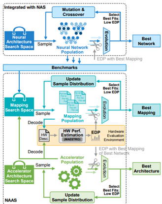
- NAAS: Neural Accelerator Architecture Search by MIT (Han Lab) (https://arxiv.org/pdf/2105.13258v1.pdf).The paper proposes a NAAS method that holistically searches the neural network architecture, accelerator architecture and compiler mapping in one optimization loop. NAAS composes highly matched architectures together with efficient mapping. As a data-driven approach, NAAS rivals the human design Eyeriss by 4.4×EDP reduction with 2.7% accuracy improvement on ImageNet under the same computation resource, and offers 1.4× to 3.5× EDP reduction than only sizing the architectural hyper-parameters.
Q3'22: Technology update – low precision and model optimization
Authors
Alexander Kozlov, Pablo Munoz, Vui Seng Chua, Nikolay Lyalyushkin, Yury Gorbachev, Nilesh Jain
Summary
We would characterize this quarter as “let’s go beyond INT8inference”. This quote is about “ANT”, a paper that you can find in theHighlights and that introduces 4-bit data type for accurate model inferencewhich fits well with the current HW architectures. There is also a lot of hypearound FP8 precisions that are already available in the latest Nvidia Hopperarchitecture and are being planned to be added into the next generations of Intel HW.
Highlights
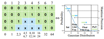
- ANT: Exploiting Adaptive Numerical Data Type for Low-bit Deep Neural Network Quantization by Microsoft Research and universities of China and US (https://arxiv.org/pdf/2208.14286.pdf). A very interesting read about a new data type for model inference which authors called flint and which combines the advantages of float and int. They proposed an encoding/decoding scheme for this type as well as the implementation of computational primitives that are based on the existing DL HW architectures. Authors also evaluate the computational efficiency of the type and show the accuracy of using it for inference on a diverse set of models.
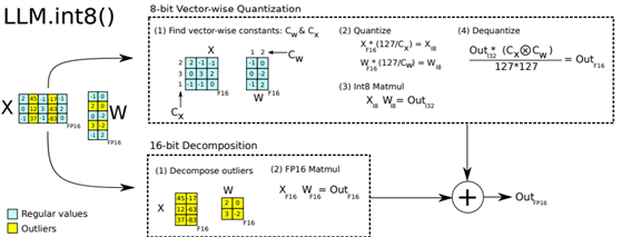
- LLM.int8(): 8-bit Matrix Multiplication for Transformers at Scale by the collaboration of Facebook, HuggingFace and universities (https://arxiv.org/pdf/2208.07339v1.pdf). The main idea of the proposed method is to split matrix multiplication operation (MatMul) which is the main operation of Transformer-based models into two separate MatMuls. The one is quantized to 8-bits and another is kept to FP16 precision. The result of both operations is summed. This mixed-precision decomposition for MatMul is based on a magnitude criterium. The authors achieved good results in accelerating of Transformer models on Nvidia GPUs. Code is available at: https://github.com/TimDettmers/bitsandbytes.
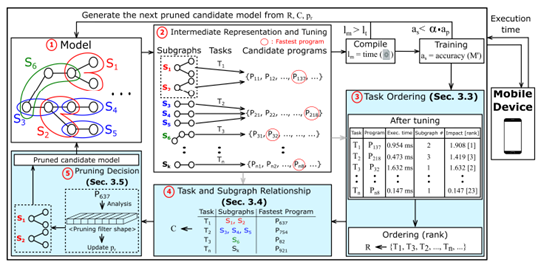
- CPrune: Compiler-Informed Model Pruning for Efficient Target-Aware DNN Execution by University of Colorado Boulder and Electronics and Telecommunications Research Institute (https://arxiv.org/pdf/2207.01260.pdf). The paper proposes a method, which incorporates the information extracted during the compiler optimization process into creating a target-oriented compressed model fulfilling accuracy requirements. This information also reduces the search space for parameter tuning. The code is available at: https://github.com/taehokim20/CPrune.
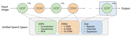
- UniNet: Unified Architecture Search with Convolution, Transformer, and MLP by MMLab and SenseTime (https://arxiv.org/pdf/2207.05420.pdf). Authors construct the search space and study the learnable combination of convolution, transformer, and MLP integrating it into an RL-based search algorithm. They conclude that: (1) placing convolutions in the shallow layers and transformers in the deep layers, (2) allocating a similar amount of FLOPs for both convolutions and transformers, and (3) inserting a convolution-based block to downsample for convolutions and a transformer-based block for transformers. The best model achieves 87.4% top1 on ImageNet outperforming Swin-L. Code will be available at https://github.com/Sense-X/UniNet.
Papers with notable results
Quantization
- I-ViT: Integer-only Quantization for Efficient Vision Transformer Inference by universities of China (https://arxiv.org/pdf/2207.01405.pdf). Authors propose efficient approximations of non-linear functions of Transformer architecture, namely Softmax, GeLU, and LayerNorm. These approximations are used to get the integer-only computational graph. They applied the proposed method to several vision Transformer models and get close to 4x speedup when going from FP32 to INT8 computations. To get the quantized model authors used a straightforward quantization-aware training method. For all the models they got a little worse or even better accuracy.
- Sub 8-Bit Quantization of Streaming Keyword Spotting Models for Embedded Chipsets by Alexa, Amazon (https://arxiv.org/pdf/2207.06920.pdf). Some practical work on the quantization of the Keyword Spotting language models. Authors used a 2-stage QAT algorithm: for the 1st-stage, they adapt a non-linear quantization method on weights, while for the 2nd-stage, we use linear quantization methods on other components of the network. The method has been used to improve the efficiency on ARM NEON architecture, where authors obtain up to 3 times improvement in CPU consumption and more than 4 times improvement in memory consumption.
- CADyQ: Content-Aware Dynamic Quantization for Image Super-Resolution by universities of South Korea and Nvidia (https://arxiv.org/pdf/2207.10345.pdf). A practical study of applying low bit-width mixed-precision quantization to Super Resolution models. Authors proposed a pipeline of selecting different bit-width for each patch and layer of the model by adding a lightweight bit selector module that is conditioned on the estimated quantization sensitivity. They also introduce a new to find a better balance between the computational complexity and overall restoration performance. The method shows good accuracy and performance results measured on T4 GPU using 8-bit and 4-bit arithmetic. Code is available at: https://github.com/Cheeun/CADyQ.
- Bitwidth-Adaptive Quantization-Aware Neural Network Training: A Meta-Learning Approach by universities of South Korea (https://arxiv.org/pdf/2207.10188.pdf). The paper proposes a method of bitwidth-adaptive quantization aware training (QAT) where meta-learning is effectively combined with QAT by redefining meta-learning tasks to incorporate bitwidths. The method trained model to be quantized to any candidate bitwidth with minimal inference accuracy drop. The paper provides some insight on how optimization can be done in the scenarios such as Iterative Learning, task adaptation, etc.
- Efficient Activation Quantization via Adaptive Rounding Border for Post-Training Quantization by Microsoft Research and universities of Shanghai (https://arxiv.org/pdf/2208.11945.pdf). The authors explore the benefits of adjusting rounding schemes of providing a new perspective for the post-training quantization. They design a border function that produces unbiased elementwise errors and makes it can adjust to specific activations to generate adaptive rounding schemes. They experiment with ImageNet models and get promising results for 4-bit and even 2-bit quantization schemes in the post-training setup.
- FP8 Quantization: The Power of the Exponent by Qualcomm AI Research (https://arxiv.org/pdf/2208.09225.pdf). This paper investigated the PTQ and QAT efficacy of FP8 schemes by varying bit-length of Mantissa (M) and Exponent(E) and exponent bias flexibility (per channel/tensor) across a wide range of convolutional and transformer topologies and tasks. The authors concluded that multi-FP8 formats are required for translating FP-trained deep networks due to model-specific optimal dynamic range and precision trade-off. Networks (BERT, ViT, SalsaNext, HRNet) with outlying dynamic ranges require more exponent bits whereas convnets require more mantissa bits for precision. FP8 formats are also more friendly for PTQ as compared to Int8.
Pruning
- CAP: instance complexity-aware network pruning by universities of China (https://arxiv.org/pdf/2209.03534.pdf). Authors exploit the difference of instance complexity between the datase samples to boost the accuracy of pruning method. They introduce a new regularizer on the soft masks of filters, the masks of important filters are pushed towards 1 and those of redundant filters are pushed towards 0, thus a sweet spot can be easily found to separate the two parts of filters. It helped to achieve compelling results in sparsity, e.g. prune 87.75% FLOPs of ResNet50 with 0.89% top-1 accuracy loss.
- Sparse Attention Acceleration with Synergistic In-Memory Pruning and On-Chip Recomputation by Google Brain and University of California (https://arxiv.org/pdf/2209.00606.pdf). The paper proposes a HW accelerator that leverages the inherent parallelism of ReRAM crossbar arrays to compute attention scores in an approximate manner. It prunes the low attention scores using a lightweight analog thresholding circuitry within ReRAM, enabling it to fetch only a small subset of relevant data to on-chip memory. To mitigate potential negative repercussions for model accuracy, the accelerator re-computes the attention scores for the few-fetched data in digital. The combined in-memory pruning and on-chip recompute of the relevant attention scores enables transforming quadratic complexity to a merely linear one. This yields 7.5x speedup and 19.6x energy reduction when total 16KB on-chip memory is used.
- OPTIMAL BRAIN COMPRESSION: A FRAMEWORK FOR ACCURATE POST-TRAINING QUANTIZATION AND PRUNING by IST Austria & Neural Magic (https://arxiv.org/pdf/2208.11580.pdf). The paper introduces a compression framework that covers both weight pruning and quantization in a post-training setting. At the technical level, the approach is based on the first exact and efficient realization of the classical Optimal Brain Surgeon (OBS) framework at the scale of modern DNNs, which we further extend to cover weight quantization. Experimental results show it can enable the accurate joint application of both pruning and quantization at post-training.
Neural Architecture Search
- You Only Search Once: On Lightweight Differentiable Architecture Search for Resource-Constrained Embedded Platforms by universities of Singapore (https://arxiv.org/pdf/2208.14446.pdf). The paper introduces an accurate predictor to estimate the latency of the architecture (𝑎𝑟𝑐ℎ). The arch is encoded with a sparse matrix 𝛼 ∈ {0, 1} 𝐿×𝐾, where the element indicates that the 𝑘-th operator is reserved for the 𝑙-th layer of 𝑎𝑟𝑐ℎ. The latency predictor is an MLP model (3 FC layers) where the input is a flattened 𝛼. The authors also propose a lightweight differentiable search method to reduce the optimization complexity to the single-path level. They compare with other popular methods such as OFA, MNAS, FBNAS, etc., and report superior results. The code is available here: https://github.com/stepbuystep/LightNAS.
- SenseTime Research 2 Shanghai AI Lab 3Australian National University by SenseTime Research Shanghai AI Lab and Australian National University (https://arxiv.org/pdf/2207.13955.pdf). Authors employ NAS for searching for a representative model based on the cosFormer architecture. They propose a new usage of attention, namely mixing Softmax attention and linear attention in the Transformer, and define a new search space for attention search in the NAS framework. The proposed mixed attention achieves a better balance between accuracy and efficiency, i.e., having comparable performance to the standard Transformer while maintaining good efficiency.
- NASRec: Weight Sharing Neural Architecture Search for Recommender Systems by Meta AI, Duke University, and University of Houston (https://arxiv.org/pdf/2207.07187.pdf). Authors propose a paradigm to scale up automated modeling of recommender systems. The method establishes a supernet with minimal human priors, overcoming data modality and architecture heterogeneity challenges in the recommendation domain. Authors advance weight-sharing NAS to the recommendation domain by introducing single-operator any-connection sampling, operator balancing interaction modules, and post-training fine-tuning. The method outperforms both manually crafted models and models discovered by NAS methods with smaller search cost.
- Tiered Pruning For Efficient Differentiable inference-aware Neural Architecture search by NVidia (https://arxiv.org/pdf/2209.11785.pdf). Authors propose three pruning techniques to improve the cost and results of Differentiable Neural Architecture Search (DNAS). Instead of evaluating all possible parameters, they evaluate just two which converge to a single optimal one (e.g. to optimal number of channels in Inverted Residual Blocks). Progressively remove blocks from the search space which are rarely chosen during SuperNet training. Skip connection is not present in the search space at the beginning of search and is inserted after removing the penultimate block of the layer in its place. The proposed algorithm establishes a new state-of-the-art Pareto frontier for NVIDIA V100 in terms of inference latency for ImageNet Top-1 image classification accuracy.
- When, where, and how to add neurons to ANNs (https://arxiv.org/pdf/2202.08539v2.pdf). Authors propose an novel approach to search for neural architectures using structural learning, and in particular neurogenesis. A framework is introduced in which triggers and initializations are used for studying the various facets of neurogenesis: when, where, and how to add neurons during the learning process. The neurogenesis strategies, termed Neural Orthogonality (NORTH*), combine, “layer-wise triggers and initializations based on the orthogonality of activations or weights to dynamically grow performant networks that converge to an efficient size”. The paper offers relevant insights that can be used in more broader Neural Architecture Search frameworks.
Other
- On-Device Training Under 256KB Memory by MIT (https://arxiv.org/pdf/2206.15472.pdf). Authors propose Quantization-Aware Scaling to calibrate the gradient scales and stabilize quantized training. To reduce the memory footprint, they introduce Sparse Update to skip the gradient computation of less important layers and sub-tensors. The algorithm is implemented by a lightweight training system, Tiny Training Engine, which prunes the backward computation graph to support sparse updates and offload the runtime auto-differentiation to compile time. Method is available at: https://github.com/mit-han-lab/tinyengine.
Deep Learning Software
- Efficient Quantized Sparse Matrix Operations on Tensor Cores (https://arxiv.org/pdf/2209.06979.pdf). A high-performance sparse-matrix library for low-precision integers on Tensor cores. Magicube supports SpMM and SDDMM, two major sparse operations in deep learning with mixed precision. Experimental results on an NVIDIA A100 GPU show that Magicube achieves on average 1.44x (up to 2.37x) speedup over the vendor-optimized library for sparse kernels, and 1.43x speedup over the state-of-the-art with a comparable accuracy for end-to-end sparse Transformer inference.
- A BetterTransformer for Fast Transformer Inference. PyTorch introduced the support of new operations that improve inference of Transformer models and can “take advantage of sparsity in the inputs to avoid performing unnecessary operations on padding tokens”.
Deep Learning Hardware
- NVIDIA, Arm, and Intel Publish FP8 Specification for Standardization as an Interchange Format for AI (blog post). The precision is already available in the latest Nvidia Hopper architecture and is planned in all the Intel HW.
CPU Dispatcher Control for OpenVINO™ Inference Runtime Execution
Introduction
CPU plugin of OpenVINO™ toolkit as one of the most important part, which is powered by oneAPI Deep Neural Network Library (oneDNN) can help user achieve high performance inference of neural networks on Intel®x86-64 CPUs. The CPU plugin detects the Instruction Set Architecture (ISA) in the runtime and uses Just-in-Time (JIT) code generation to deploy the implementation optimized for the latest supported ISA.
In this blog, you will learn how layer primitives been optimized by implementation of ISA extensions and how to change the ISA extensions’ optimized kernel function at runtime for performance tuning and debugging.
After reading this blog, you will start to be proficient in AI workloads performance tuning and OpenVINO™ profiling on Intel® CPU architecture.
CPU Profiling
OpenVINO™ provide Application Program Interface (API) which is easy to turn on CPU profiling and analyze performance of each layer from the bottom level by executed kernel function. Firstly, enable performance counter profiling with executed device during device property configuration before model compiling with device. Learn detailed information from document of OpenVINO™ Configuring Devices.
Then, you are allowed to get object of profiling info from inference requests which complied with the CPU device plugin.
Please note that performance profiling information generally can get after model inference. Refer below code implementation and add this part after model inference. You are possible to get status and performance of layer execution. Follow below code implement, you will get performance counter printing in order of the execution time from largest to smallest.
CPU Dispatching
By enabling device profiling and printing exec_type of layers, you will get the specific kernel functions which powered by oneDNN during runtime execution. Use TensorFlow* ResNet 50 INT8 model for execution and pick the first 10 hotspot layers on 4th Gen Intel® Xeon Scalable processor (code named Sapphire Rapids) as an example:
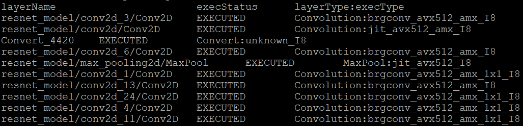
From execution type of layers, it would be helpful to check which oneDNN kernel function used, and the actual precision of layer execution and the optimization from supported ISA on this platform.
Normally, oneDNN is able to detect to certain ISA, and OpenVINO™ allow to use latest ISA with higher priority. If you want to compare optimization rate between different ISA, can use the ONEDNN_MAX_CPU_ISA environment variable to limit processor features with older instruction sets. Follow this link to check oneDNN supported ISA.
Please note, Intel® Advanced Matrix Extensions (Intel® AMX) ISA start to be supported since 4th Gen Intel® Xeon Scalable processor. You can refer Intel® Product Specifications to check the supported instruction set of your current platform.
The ISAs are partially ordered:
· SSE41 < AVX < AVX2 < AVX2_VNNI <AVX2_VNNI_2,
· AVX2 < AVX512_CORE < AVX512_CORE_VNNI< AVX512_CORE_BF16 < AVX512_CORE_FP16 < AVX512_CORE_AMX <AVX512_CORE_AMX_FP16,
· AVX2_VNNI < AVX512_CORE_FP16.
To use CPU dispatcher control, just set the value of ONEDNN_MAX_CPU_ISA environment variable before executable program which contains the OpenVINO™ device profiling printing, you can use benchmark_app as an example:
The benchmark_app provides the option which named “-pcsort” can report performance counters and order analysis information by order of layers execution time when set value of the option by “sort”.
In this case, we use above code implementation can achieve similar functionality of benchmark_app “-pcsort” option. User can consider try to add the code implementation into your own OpenVINO™ program like below:
After setting the CPU dispatcher, the kernel execution function has been switched from AVX512_CORE_AMX to AVX512_CORE_VNNI. Then, the performance counters information would be like below:
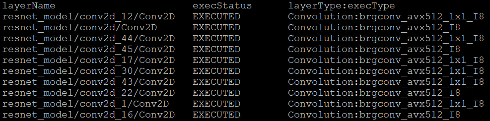
You can easily find the hotspot layers of the same model would be changed when executed by difference kernel function which optimized by implementation of different ISA extensions. That is also the optimization differences between architecture platforms.
Tuning Tips
Users can refer the CPU dispatcher control and OpenVINO™ device profiling API to realize performance tuning of your inference program between CPU architectures. It will also be helpful to developer finding out the place where has the potential space of performance improvement.
For example, the hotspot layer generally should be compute-intensive operations like matrix-matrix multiplication; General vector operations which is not target to artificial intelligence (AI) / machine learning (ML) workloads cannot be optimized by Intel® AMX and Intel® Deep Learning Boost (Intel® DL Boost), and the memory accessing operations, like Transpose which maybe cannot parallelly optimized with instruction sets. If your inference model remains large memory accessing operations rather than compute-intensive operations, you probably need to be focusing on RAM bandwidth optimization.
Automatic Device Selection and Configuration with OpenVINO™
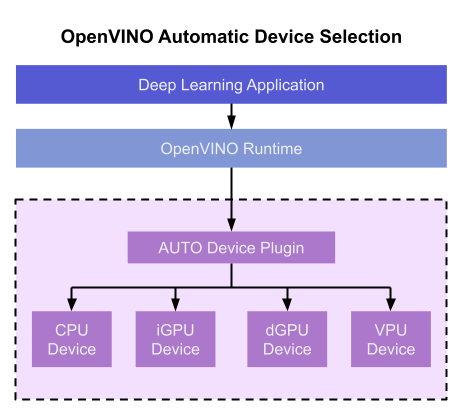
OpenVINO empowers developers to write deep learning application code once and deploy it on a wide range of Intel hardware with best-in-class performance. Previously, significant effort had to be spent configuring inference pipelines to squeeze optimal performance out of target hardware, and the effort had to be repeated whenever the application was ported to a new platform. The new Auto Device Plugin (AUTO) and automatic configuration features in OpenVINO make it easier for developers to unlock performance on multiple hardware targets without needing to spend time optimizing their application pipeline.
When an OpenVINO application is deployed in a system, the Auto Device Plugin automatically selects the best hardware target to inference the model with. OpenVINO then automatically configures the application to use optimal pipeline parameters based on the hardware capabilities and model size. Developers no longer need to write code for detecting hardware devices and explicitly configuring batch and stream parameters. High-level configuration is provided through performance hints that allow a developer to prioritize their application for either high throughput or minimal latency. AUTO and automatic device configuration make applications hardware-agnostic, allowing them to easily be ported to new hardware without any code changes.
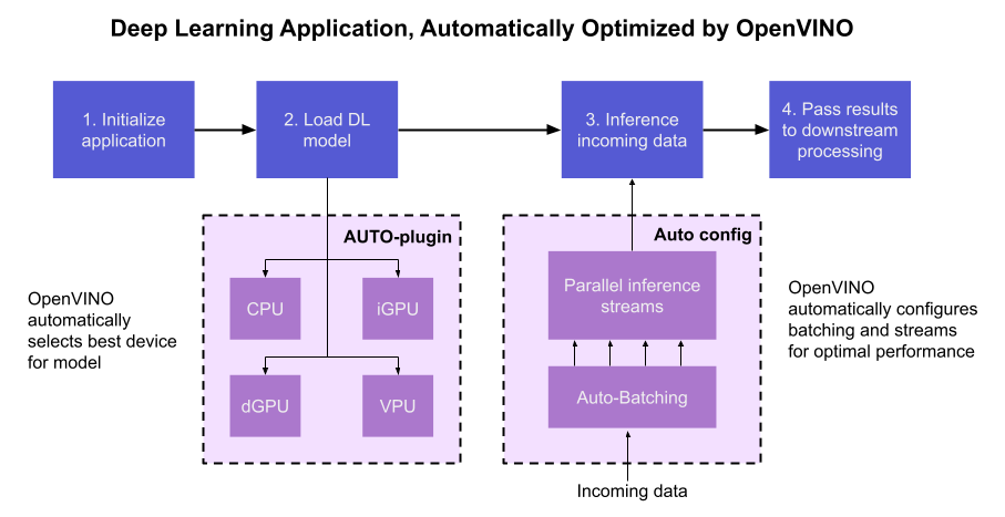
The diagram in Figure 1 shows how OpenVINO’s features automatically configure an application for optimal performance, regardless of the target hardware. When the deep learning model is loaded, AUTO creates a transparent plugin interface to the available processor devices and automatically selects the most suitable device. OpenVINO configures the batch size and number of processing streams based on the selected hardware target, and the Auto-Batching feature automatically groups incoming data into optimally sized batches. AUTO and automatic configuration operate independently from each other, so developers can use either or both in their application.
AUTO and automatic configuration are available starting in the 2022.1 release of OpenVINO Runtime. To use these features, simply install OpenVINO Runtime on the target hardware. The API uses AUTO by default if no processor device is specified when loading a model. Set a “throughput” or “latency” performance hint when loading the model, and the API automatically configures the inference pipeline. Read on to learn more about AUTO, automatic configuration, performance hints, and how to use them in your application.
Automatic Device Selection
Auto Device Plugin (AUTO) is a “virtual” device that provides a transparent interface to physical devices in the system. When an application is initialized, AUTO discovers the available processors and accelerators in the system (CPUs, integrated GPUs, discrete GPUs, VPUs) and selects the best device, based on a default device priority list or an optional user-provided priority list. It creates an interface between the application and device that executes inference requests in an optimized fashion. It enables an application to always achieve optimal performance in a system without the developer having to know beforehand what devices are available in the system.
Key Features and Benefits
Simple and flexible application deployment
Previously, developers needed to know details about target hardware and configure their application specifically for each device. AUTO removes the need to write dedicated code for specific devices. This enables an application to be written once and deployed to any supported hardware. It also allows the application to run on newer generations of hardware as they are released: the developer only needs to compile the application with the latest version of OpenVINO to run it on new hardware. This provides an instant increase in performance with little development time.
Configurability
AUTO provides a configuration interface that is easy to use at a high level while still providing flexibility. Developers can simply specify “AUTO” as the device to tell the application to select the best device for the given model. They can also control which device is selected by providing a device candidate list and setting priorities for each device.
Developers can also use performance hints to configure their application for latency or throughput. When the performance hint is throughput, OpenVINO will create more streams for parallel inferencing to achieve maximum processing bandwidth. In latency mode, OpenVINO creates fewer streams to utilize as many resources as possible to complete each inference quickly. Performance hints also help determine the optimal batch size for inferencing; this is discussed further in the “Performance Hints” section of this document.
Improved first-inference latency
In applications that use accelerated processors like GPUs or VPUs, the time to first inference may be higher than average because it takes time to compile and load the deep learning model into the accelerator. AUTO solves this problem by starting the first inference with the CPU, which has minimal latency and no delays. As the first inference is being performed, AUTO continues to compile and load the model for the selected accelerator device, and then transparently switches over to that device when it is ready. This significantly reduces time to first inference, and is beneficial for applications that require immediate inference results on startup.
How Automatic Device Selection Works
To choose the best device for inference, AUTO discovers which hardware targets are available in the system and matches the model to the best supported device, using the following process:
- AUTO discovers which devices are available using the Query Device API. The query reads an internal file that lists installed hardware plugins, confirms the hardware modules are present by communicating with them through drivers, and returns a list of available devices in the system.
- AUTO checks the precision of the input model by reading the model file.
- AUTO selects the best available device in the device priority table (shown in Table 1 below) that is capable of supporting the model’s precision.
- AUTO attempts to compile the model on the selected device. If the model doesn’t compile (for example, if the device doesn’t support all the operations required by the model), AUTO tries to compile it on the next best device until compilation is successful. The CPU is the final fallback device, as it supports all operations and precisions.
By default, AUTO uses the device priority list shown in Table 1. Developers can customize the table to provide their own device priority list and limit the devices that are available to run inferencing. AUTO will not try to run inference on devices that are not provided in the device list.
Table 1. Default AUTO Device Priority List
As mentioned, AUTO reduces the first inference latency by compiling and loading the model to the CPU first. As the model is loaded to the CPU and first inference is performed, AUTO steps through the rest of the process for selecting the device and compiling the model to that device. This way, devices that require a long time for model compilation do not impede inference as the application is being initialized.
AUTO also provides a model priority feature that enables developers to control which models are loaded to which devices when there are multiple models running on a system with multiple devices. Developers can set “MODEL_PRIORITY” as “HIGH”, “MEDIUM”, or “LOW” to configure which models should be allocated to the best resource. This allows developers to ensure models that are critical for an application are always loaded to the fastest device for processing, while less critical models are loaded to slower devices.
For example, consider a medical imaging application with models for segmenting and/or classifying injuries in X-ray images running on a system that has both a GPU and a CPU. The segmentation model is set to HIGH priority because it takes more processing power to inference, while the classification model is set to MEDIUM priority. If both models are loaded at the same time, the segmentation model will be loaded to the GPU (the higher priority device) and the classification model will be loaded to the CPU (the lower priority device). If only the classification model is loaded, it will be loaded to the GPU since the GPU isn’t occupied by the higher-priority model.
Automatic Device Configuration
The performance of a deep learning application can be improved by configuring runtime parameters to fully utilize the target hardware. There are several factors to take into consideration when optimizing inference for a certain device, such as batch size and number of streams. (See Runtime Inference Optimizations in OpenVINO documentation for more information.) The optimal configuration for these parameters depends on the architecture and memory of the target hardware, and they need to be re-determined when porting an application from one device to another.
OpenVINO provides features that automatically configure an application to use optimal runtime parameters to achieve the best performance on any supported hardware target. These features are enabled through performance hints, which allow a user to specify whether their application should be optimized for latency or throughput. The automatic configuration eliminates the time and effort required to determine optimal configurations. It makes it simple to port to new devices or write one application to work on multiple devices. OpenVINO’s automatic configuration features currently work with CPU and GPU devices, and support for VPUs will be added in a future release.
Performance Hints
OpenVINO allows users to provide high-level "performance hints" for setting latency-focused or throughput-focused inference modes. These performance hints are “latency” and “throughput.” The hints cause the runtime to automatically adjust runtime parameters, such as number of processing streams and inference batch size, to prioritize for reduced latency or high throughput. Performance hints are supported by CPU and GPU devices, and a future release of OpenVINO will add support for VPUs.
The performance hints do not require any device-specific settings and are portable between devices. Parameters are automatically configured based on whichever device is being used. This allows users to easily port applications between hardware targets without having to re-determine the best runtime parameters for the new device.
Latency performance hint
Latency is the amount of time it takes to process a single inference request and is usually measured in milliseconds (ms). In applications where data needs to be inferenced and acted on as quickly as possible (such as autonomous driving), low latency is desirable. When applications are run with the “latency” performance hint, OpenVINO determines the optimal number of parallel inference requests for minimizing latency while still maximizing the parallelization capabilities of the hardware. It automatically sets the number of processing streams to achieve the best latency.
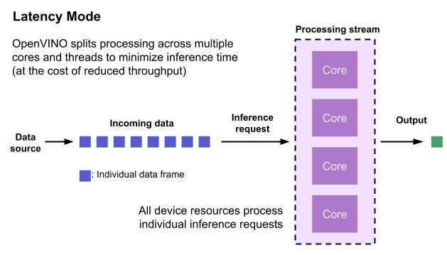
To achieve the fastest latency, the processor device should process only one inference request at a time so all the compute resources are available for calculation. However, devices with multiple cores (such as multi-socket CPUs or multi-tile GPUs) can deliver multiple streams with the same latency as they would with a single stream. OpenVINO automatically checks the compute demands of the model, queries capabilities of the device, and selects the number of streams to be the minimum required to get the best latency. For CPUs, this is typically one stream for each socket. For GPUs, it’s typically one stream per tile.
Throughput performance hint
Throughput is the amount of data an inferencing pipeline can process at once, and it is usually measured in frames per second (FPS) or inferences per second. In applications where large amounts of data needs to be inferenced simultaneously (such as multi-camera video streams), high throughput is needed. To achieve high throughput, the runtime should focus on fully saturating the device with enough data to process. When applications are run with the “throughput” performance hint, OpenVINO maximizes the number of parallel inference requests to utilize all the threads available on the device. On GPU, it automatically sets the inference batch size to fill up the GPU memory available.
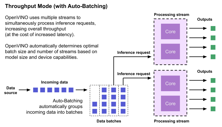
To configure the runtime for high throughput, OpenVINO automatically sets the number of streams to use based on the architecture of the device. For CPUs, it creates as many streams as there are cores available. For GPUs, it uses a combination of batch size and parallel streams to fully utilize the GPU’s memory and compute resources. To determine the optimal configuration on GPUs, OpenVINO will first check if the network supports batching. If it does, it loads the network with a batch size of one, determines how much memory is used for the single-batch network, and then scales the batch size and streams up to fill the entire GPU.
Batch size can also be explicitly specified in code when the model is loaded. This can be useful in applications where the number of incoming data sources is known and constant. For example, in an application that processes four camera streams, specify a batch size of four so that each set of frames from the cameras is processed in a single inference request. More information on batch configuration is given in the Auto-Batching section below.
Auto-Batching
Auto-Batching is a new feature of OpenVINO that performs on-the-fly grouping of data inference requests in an application. As the application makes individual inference requests, Auto-Batching transparently collects them into a batch. When the batch is full (or when a timeout limit is reached), OpenVINO executes inference on the whole batch. In short, it takes care of batching data efficiently so the developer doesn’t have to worry about it.
The Auto-Batching feature is controlled by the configuration parameter “ALLOW_AUTO_BATCHING”, which is enabled by default. Auto-Batching is activated when all of the following are true:
- ALLOW_AUTO_BATCHING is true
- The model is loaded to the target device with the throughput performance hint
- The target device supports batching (such as GPU)
- The model topology supports batching
When Auto-Batching is activated, OpenVINO automatically determines the optimal batch size for an application based on model size and hardware capabilities. Developers can also explicitly specify the batch size when loading the model. While the inference pipeline is active, individual inference requests are gathered into a batch and then executed when the batch is full.
Auto-Batching also has a timeout feature that is configurable by the developer. If there aren’t enough individual requests collected within the developer-specified time limit, batch execution will fall back to just using individual inference requests. For example, a developer may specify a timeout limit of 500 ms and a batch size of 16 for a video processing inference pipeline. Once 16 frames are gathered, a batch inference request is made. If only 13 frames arrive before the 500 ms timeout is hit, the application will perform individual inference requests on each of the 13 frames. While the timeout feature makes the pipeline robust to interruptions in incoming data, hitting the timeout limit heavily reduces the performance. To avoid this, developers should make sure there is enough incoming data to fill the batch within the time limit in typical conditions.
Auto-Batching, when combined with OpenVINO's automatic configuration features that determine optimal batch size and number of streams, provides a powerful benefit to the developer. The developer can utilize the full power of the target device with only using one line of code. Best of all, when an application is used on a different device, it will automatically reconfigure itself to achieve optimal performance with zero effort from the developer.
How to Use AUTO and Performance Hints
Using AUTO and automatic configuration with performance hints only requires one line of code. The functionality centers around the “ie.compile_model” method, which is used to compile a model and load it into device memory. The method accepts various configuration parameters that allow a user to provide high-level control over the pipeline.
Here are several Python examples showing how to configure a model and pipeline with the ie.compile_model method. The first example also shows how to import the OpenVINO Core model, initialize it, and read a model before calling ie.compile_model.
Example 1. Load a model on AUTO device
Example 2. Load a model on AUTO device with performance hints
Example 3. Provide a list of device candidates which AUTO may use when loading a model
Example 4. Load multiple models with HIGH, MEDIUM, and LOW priorities
Example 5. Load a model to GPU and use Auto-Batching with an explicitly set batch size
For a more in-depth example of how to use AUTO and automatic configuration, please visit the Automatic Device Selection with OpenVINO Jupyter notebook in the OpenVINO notebooks repository. It provides an end-to-end example that shows:
- How to download a model from Open Model Zoo and convert it to OpenVINO IR format with Model Optimizer
- How to load a model to AUTO device
- The improvement in first inference latency when using AUTO device
- How to perform asynchronous inferencing on data batches in throughput or latency mode
- A performance comparison between throughput and latency modes
The OpenVINO Benchmark App also serves as a useful tool for experimenting with devices and batching to see how performance changes under various configurations. The Benchmark App supports automatic device selection and performance hints for throughput or latency.
Where to Learn More
To learn more please visit auto device plugin and automatic configuration pages in OpenVINO documentation. They provide more information about how to use and configure them in an application.
OpenVINO also provides an example notebook explaining how to use AUTO and showing how it improves performance. The notebook can be downloaded and run on a development machine where OpenVINO Developer Tools have been installed. Visit the notebook at this link: Automatic Device Selection with OpenVINO.
To learn more about OpenVINO toolkit and how to use it to build optimized deep learning applications, visit the Get Started page. OpenVINO also provides a number of example notebooks showing how to use it for basic applications like object detection and speech recognition on the Tutorials page.

Introducing OpenVINO™ integration with TensorFlow*
ArindamViral adoption of technologies is often triggered by leaps in user experience. For example, the iPhone prompted the rapid adoption of smartphones and the “app store.” Or, more recently, the ease of use seen in TensorFlow kickstarted the massive growth of Artificial Intelligence that touches almost every aspect of our daily lives today.
OpenVINO™ toolkit has redefined AI inferencing on Intel powered devices and has attained unprecedented developer adoption. Today hundreds of thousands of developers use OpenVINO™ toolkit to accelerate AI inferencing across almost all imaginable use cases, from emulation of human vision, automatic speech recognition, natural language processing, recommendation systems, and many others. Based on latest generations of artificial neural networks, including Convolutional Neural Networks (CNNs), recurrent and attention-based networks, the toolkit extends computer vision and non-vision workloads across Intel® hardware (Intel® CPU, Intel® Integrated Graphics, Intel® Neural Compute Stick 2, and Intel® Vision Accelerator Design with Intel® Movidius™ VPUs), maximizing performance. It accelerates applications with high-performance, AI, and deep learning inference deployed from edge to cloud.
We are honored to partner with our customers and contribute to their success. We are constantly listening and innovating to meet their evolving needs while also aiming to provide a world class user experience. Therefore, based on customer feedback, and building on OpenVINO™ toolkit’s success, we are introducing the OpenVINO™ integration with TensorFlow*. This integration enables TensorFlow developers to accelerate inferencing of their TensorFlow models in deployment with just 2 additional lines of code.
Benefits for TensorFlow Developers:
OpenVINO™ integration with TensorFlow* delivers OpenVINO™ toolkit inline optimizations and runtime needed for an enhanced level of TensorFlow compatibility. It is designed for developers who would like to experience the benefits of using OpenVINO™ toolkit – help boost performance for their inferencing applications – with minimal code modifications. It accelerates inference across many AI models on a variety of Intel® silicon, such as:
- Intel® CPU
- Intel® Integrated Graphics
- Intel® Movidius™ Vision Processing Units - referred as VPU
- Intel® Vision Accelerator Design with 8 Intel Movidius™ MyriadX VPUs - referred as VAD-M or HDDL
Developers leveraging this integration can expect the following benefits:
- Performance acceleration compared to native TensorFlow (depending on underlying hardware configuration).
- Accuracy – preserve accuracy nearly identical to original model.
- Simplicity – Continue to use TensorFlow APIs for inferencing. No need to refactor code. Just import, enable, and set device.
- Robustness – architected to support a wide range of TensorFlow models and operators across a variety of OS/Python environments.
- Seamless, inline model conversions – no explicit model conversion required.
- Lightweight footprint – minimal incremental memory and disk footprint required.
- Support for broad range of Intel powered devices – CPUs, iGPUs, VPUs (Myriad-X).
[Note: For maximum performance, efficiency, tooling customization, and hardware control, we recommend going beyond this component to adopt native OpenVINO™ APIs and its runtime.]
How does it work?
Developers can greatly accelerate the inferencing of their TensorFlow models by adding the following two lines of code to their Python code or Jupyter Notebooks.
import openvino_tensorflow
openvino_tensorflow.set_backend('<backend_name>')
Supported backends include 'CPU', 'GPU', 'MYRIAD', and 'VAD-M'. See Figure 1.
Sample code:
Here is an example of OpenVINO™ integration with TensorFlow* at work:
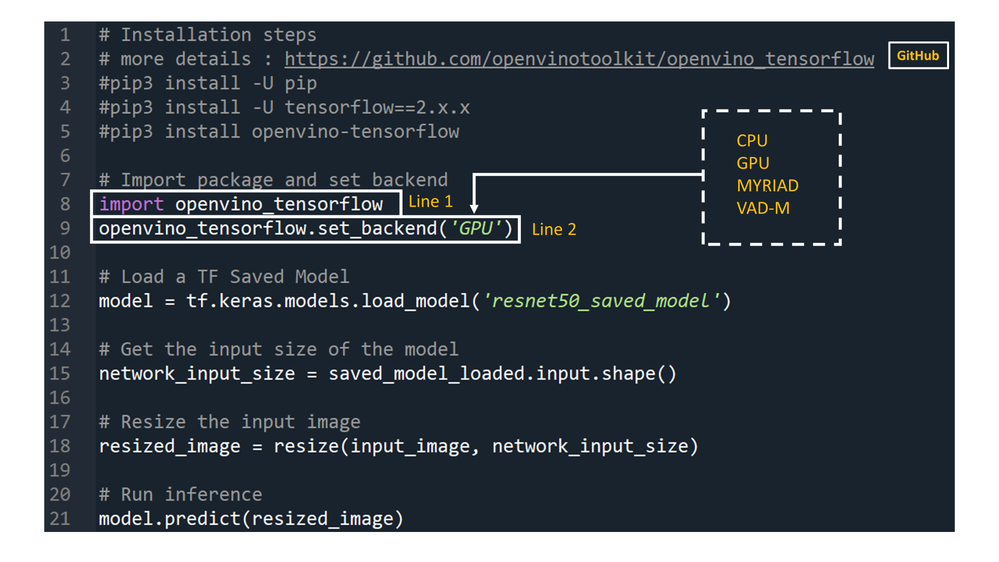
Figure 1
How does it really work under the hood?
OpenVINO™ integration with TensorFlow* provides accelerated TensorFlow performance by efficiently partitioning TensorFlow graphs into multiple subgraphs, which are then dispatched to either the TensorFlow runtime or the OpenVINO™ runtime for optimal accelerated inferencing. The results are finally assembled to provide the final inference results.
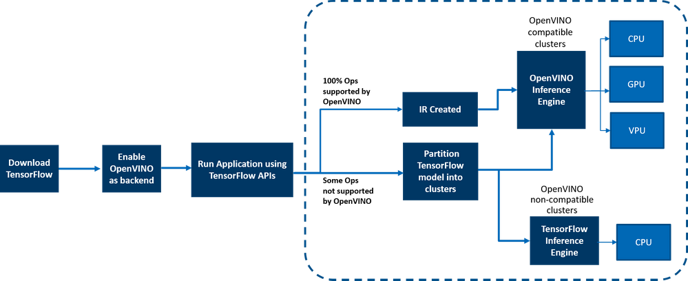
Figure 2: End-to-end overview of the workflow
Here is a detailed architecture diagram.
Deployment at the Edge and the Cloud
OpenVINO™ integration with TensorFlow* works in a variety of environments – from the cloud to the edge – as long as the underlying hardware is an Intel platform. E.g., the add-on works on the following cloud platforms:
- Intel® DevCloud for the Edge
- AWS Deep Learning AMI Ubuntu 18 & Ubuntu 20 on EC2 C5 instances optimized for inferencing
- Azure ML
- Google colab
Any AI based Edge device is supported.
Samples are available in the examples/ directory in the gitrepo.
How is this different from using native OpenVINO™ toolkit:
OpenVINO™ integration with TensorFlow* enables TensorFlow developers to accelerate their TensorFlow model inferencing in a very quick and easy manner – with just 2 lines of code. The OpenVINO™ model optimizer accelerates inference performance, along with a wealth of integrated developer tools and advanced features, but as mentioned earlier, for maximum performance, efficiency, tooling customization, and hardware control, we recommend native OpenVINO™ APIs and its runtime.
Customer adoption
Customers are using OpenVINO™ integration for TensorFlow for a variety of use cases. Here are a few examples
- Extreme Vision: Dedicated AI-only clouds such as Extreme Vision’s CV MART helps enable hundreds of thousands of developers with a rich catalog of services, models, and frameworks to further optimize their AI workloads on a variety of Intel platforms such as CPUs and iGPUs. An easy-to-use developer toolkit to accelerate models, properly integrated with AI frameworks, such as OpenVINO™ integration with TensorFlow*, provides the best of both worlds – an increase in inference speed as well as the ability to reuse already created AI inference code with minimal changes. The Extreme Vision team is testing OpenVINO™ integration with TensorFlow* with the goal of enabling TensorFlow developers on the Extreme Vision platform.
- Genome Analysis Toolkit (GATK) developed by the Broad Institute is one of the world’s most widely used open-source toolkit for variant calling. Terra is a more secure, scalable, open-source platform for biomedical researchers to access data, run analysis tools and collaborate. The cloud-based platform is co-developed by the Broad Institute of MIT and Harvard, Microsoft, and Verily. Terra platform includes GATK tools and pipelines for the research community to run their analytics. CNNScoreVariants is one of the deep learning tools included in GATK which apply a Convolutional Neural Net to filter annotated variants. In a blog, Broad Institute showcase’s how to further accelerate inference performance of CNNScoreVariants using OpenVINO™ integration with TensorFlow*.
Conclusion
Now that you have a better understanding of the benefits, how it works, deployments environments, and how OpenVINO integration with TensorFlow differs from using native OpenVINO APIs, we can’t wait for you to try OpenVINO integration with TensorFlow for yourself and begin experiencing a boost in inference performance of your AI models on all Intel platforms. And as always, we would love to hear your feedback on this integration, please contact us at OpenVINO-tensorflow@intel.com or raise issues in the gitrepo. Thank you!
Resources
Here are resources to help you learn more:

OpenVINO Execution Provider for ONNX Runtime – Same Docker Container, Different Channel
Docker containers can help you deploy deep learning models easily on different devices. With the OpenVINO Execution Provider for ONNX Runtime docker container, you can run deep learning models easily on different Intel® hardware that Intel® Distribution of OpenVINO™ Toolkit supports with the added benefit of not having to install any dependencies. Just in case you haven’t heard about OpenVINO Execution Provider for ONNX Runtime before, the OpenVINO Execution Provider for ONNX Runtime enables ONNX models for running inference using ONNX Runtime API’s while using OpenVINO™ toolkit as a backend.
Now that you know about OpenVINO Execution Provider for ONNX RT, you must be wondering how you can get your hands on it and try it out. In our previous blog, you learned about OpenVINO Execution Provider for ONNX Runtime in depth and tested out some of the object detection samples that we created. Over time, Docker Containers have become essential for AI development and we, at Intel, are aware of that. In the past, many of you have gotten access to OpenVINO Execution Provider for ONNX Runtime docker image through Microsoft’s Container Registry. Now, things are going to be a little different. We are happy to announce that the OpenVINO Execution Provider for ONNX Runtime Docker Image is now LIVE on Docker Hub.
You will still get full access to OpenVINO Execution Provider but going forward keep an eye on Docker Hub as newer versions of the Docker Image will be released there with latest and even better features. With just a simple docker pull, you will be able to accelerate inferencing of ONNX models and get that extra performance boost you’re looking for. To learn more about the latest features that OpenVINO Execution Provider has, you can check out the release notes here. If you want to learn more about how the docker container works and how to use it, please keep reading ahead.
How to Install
Prerequisites
Ubuntu/Cent-OS Linux Machine
Installation
Step 1: Downloading the docker image on the host machine
docker pull openvino/onnxruntime_ep_ubuntu18
Step 2: Running the container.
docker run -it --rm --device-cgroup-rule='c 189:* rmw' -v /dev/bus/usb:/dev/bus/usb openvino/onnxruntime_ep_ubuntu18:latest
Reference: https://hub.docker.com/r/openvino/onnxruntime_ep_ubuntu18
Video embeds must follow Webflow Guidelines
Other ways to install OpenVINO Execution Provider for ONNX Runtime
There are also other ways to install the OpenVINO Execution Provider for ONNX Runtime. One such way is to build from source. By building from source, you will also get access to C++, C# and Python API’s. Another way to install OpenVINO Execution Provider for ONNX Runtime is to install the Python wheel package via pip.