

OpenVINO Blog
Optimizing Latent Consistency Model for Image Generation with OpenVINO™ and NNCF
Authors: Liubov Talamanova, Ekaterina Aidova, Alexander Kozlov
Introduction
Latent Diffusion Models (LDMs) make a revolution in AI-generated art. This technology enables creation of high-quality images simply by writing a text prompt. While LDMs like Stable Diffusion are capable of achieving the outstanding quality of generation, they often suffer from the slowness of the iterative image denoising process. Latent Consistency Model (LCM) is an optimized version of LDM. Inspired by Consistency Models (CM), Latent Consistency Models (LCMs) enabled swift inference with minimal steps on any pre-trained LDMs, including Stable Diffusion. The Consistency Models is a new family of generative models that enables one-step or few-step generation. More details about the proposed approach and models can be found using the following resources: project page, paper, original repository.
Similar to original Stable Diffusion pipeline, the LCM pipeline consists of three important parts:
- Text Encoder to create a condition to generate an image from a text prompt.
- U-Net for step-by-step denoising latent image representation.
- Autoencoder (VAE) for decoding latent space to image.

In this post we explain how to optimize the LCM inference by OpenVINO for Intel hardware. Since LCM is trained in a way that it should be resistant to perturbations, it means that we can also apply common optimization methods such as quantization to lower the precision while expecting a consistent generation result and we do apply 8-bit Post-training Quantization from Neural Network Compression Framework (NNCF).
Convert models to OpenVINO format
To leverage efficient inference with OpenVINO runtime on the intel platform, the original model should be converted to OpenVINO Intermediate Representation (IR). OpenVINO supports the conversion of PyTorch models directly via Model Conversion API. ov.convert_model function accepts instance of PyTorch model and example inputs for tracing and returns object of ov.Model class, ready to use or save on disk using ov.save_model function. You can find conversion details of LCM in the OpenVINO LCM Notebook.
Processing time of the diffusion model
The diffusion pipeline requires multiple iterations to generate an image. Each iteration requires a non-negligible amount of time, depending on your inference device. We have benchmarked the stable diffusion pipeline on an Intel(R) Core(TM) i9-10980XE CPU @ 3.00GHz. The number of iterations was set at 10.
Benchmarking results:
Average Latency : 6.54 seconds
Encoding Phase:
Text encoding: 0.05 seconds
Denoising Loop : 4.28 seconds
U-Net part (4 iterations): 4.27 seconds
Scheduler: 0.01 seconds
Decoding Phase:
VAE decoding: 2.21 seconds
The U-Net part of the denoising loop takes more than 60% of the full pipeline execution time. That is why the computation cost and speed of the U-Net denoising becomes the critical path in the pipeline.
In this blog, we use Neural Network Compression Framework (NNCF) Post-Training Quantization (PTQ) API to quantize the U-Net model, which can further boost the model inference while keeping acceptable accuracy without fine-tuning. Quantizing the rest of the diffusion pipeline does not significantly improve inference performance but can lead to a substantial degradation of the accuracy.
Quantization
The quantization process includes the following steps:
- Create a calibration dataset for the quantization.
- Run nncf.quantize to obtain a quantized model.
- Save the INT8 model using ov.save_model function.
You can look at the dataset preparation for the U-Net model in OpenVINO LCM Notebook. General rules about dataset preparation you can find at OpenVINO documentation.
For INT8 quantization of LCM, we found some useful tricks to mitigate accuracy degradation caused by accuracy sensitive layers:
- The U-Net part of the LCM pipeline has a backbone with a transformer that operates on latent patches. To better preserve accuracy after NNCF PTQ, we should pass model_type=nncf.ModelType.Transformer to nncf.quantize function. It keeps several accuracy sensitive layers in FP16 precision.
- Default symmetric quantization of weights and activations also leads to accuracy degradation of LCM. We recommend using preset=nncf.QuantizationPreset.MIXED to use symmetric quantization of weights and asymmetric quantization of activations that are more sensitive and impact the generation results more. So applying asymmetric quantization to activations helps to better represent their values and leads to better accuracy with no impact on the inference latency.
- It was also discovered that the Fast Bias (error) Correction algorithm (FBC), which is a default part of NNCF PTQ, results in unexpected artifacts in the generated images. To disable FBC, we should pass advanced_parameters=nncf.AdvancedQuantizationParameters(disable_bias_correction=True) to nncf.quantize function.
Once the dataset is ready and the model object is instantiated, you can apply 8-bit quantization to it using the optimization workflow below:
Text-to-image generation

The left image was generated using the original LCM pipeline from PyTorch. The middle image was generated using the model converted to OpenVINO FP16. The right image was generated using LCM with the quantized INT8 U-Net. Input prompt is “a beautiful pink unicorn, 8k”, seed is 1234567 and the number of inference steps is 4.
If you would like to generate your own images and compare original and quantized models, you can run an Interactive demo at the end of OpenVINO LCM Notebook.

We also measured time for the image generation by LCM pipeline with input prompt “a beautiful pink unicorn, 8k”, seed is 1234567 and 4 inference steps.

*Average time across 3 independent runs.
Performance speedup PyTorch vs OpenVINO+NNCF is 1.38x.
Notices and Disclaimers:
Performance varies by use, configuration, and other factors. Learn more at www.intel.com/PerformanceIndex. Performance results are based on testing as of dates shown in configurations and may not reflect all publicly available updates. No product or component can be absolutely secure. Intel technologies may require enabled hardware, software or service activation.
The products described may contain design defects or errors known as errata which may cause the product to deviate from published specifications. Current characterized errata are available on request.
Test Configuration: Intel® Core™ i9-10980XE CPU Processor at 3.00GHz with DDR4 128 GB at 3600MHz, OS: Ubuntu 22.04.2 LTS. Tested with OpenVINO LCM Notebook.
The test was conducted by Intel on November 7, 2023.
Conclusion
In this blog, we introduced how to enable and quantize the Latent Consistency Model with OpenVINO™ runtime and NNCF:
- Proposed NNCF INT8 PTQ quantization improves performance of image generation pipeline while preserving generation quality.
- Provided OpenVINO LCM Notebook for model enabling, quantization, comparison of FP16 and INT8 model inference times and deployment with OpenVINO™ and NNCF.
As the next step, you can consider migration to a native OpenVINO C++ API for even faster generation pipeline inference and possibility to embed it into the client or edge-device application. You can find an example of such a pipeline here.
Please give a star to NNCF and OpenVINO repositories if you find them useful.
How to build and run OpenVino™ C++ Benchmark Application for Linux
Introduction
The OpenVINO™ Benchmark Application estimates deep learning inference performance on supported devices for synchronous and asynchronous modes.
NOTE: This guide describes the usage of the C++ implementation of the Benchmark Tool. For the Python implementation, refer to the Benchmark Python Tool page. The Python version is recommended for benchmarking models used in Python applications, and the C++ version is recommended for benchmarking models used in C++ applications.
In this tutorial, we will guide you through building and running the C++ implementation of the Benchmark Tool on Ubuntu with OpenVINO™ 2023.1.0 release and demonstrate its usage by benchmarking the Inception (GoogleNet) V3 deep learning model. The following steps outline the process:
- Download and Convert the Model
- Install OpenVINO™ Runtime
- Build OpenVINO™ C++ Runtime Samples
- Run the Benchmark Application
The benchmark application works with models in the OpenVINO™ IR (.xml and .bin), ONNX (.onnx), TensorFlow (*.pb), TensorFlow Lite (*.tflite) and PaddlePaddle (*.pdmodel) formats. Make sure to convert your models if necessary (see "Model conversion to OpenVINO™ IR format" step below).
Requirements
Before getting started, ensure that you have the following requirements in place:
- Ubuntu 18.04 or higher
- CMake version 3.10 or higher
Step 1: Install OpenVINO™
To get started, first install OpenVINO™ Runtime C++ API.
Download and Setup OpenVINO™ Runtime archive file for Linux for your system. The following steps describe the installation process for Ubuntu 20.04 x86_64 system:
1. Download the archive file, extract the files, rename the extracted folder, and move it to the desired path:
2. Install required system dependencies on Linux. To do this, OpenVINO provides a script in the extracted installation directory. Run the following command:
3. For simplicity, it is useful to create a symbolic link as below:
4. Set OpenVINO™ environment variables. Open a terminal window and run the setupvars.sh script to temporarily set your environment variables. If your <INSTALL_DIR> is not /opt/intel/openvino_2023, use the correct one instead:
Step 2: Build OpenVINO™ C++ Runtime Samples
In the existing terminal window where the OpenVINO™ environment is set up, navigate to the /opt/intel/openvino_2023.1.0/samples/cpp directory and run the /build_samples.sh script:
As a result of a successful build, you'll get the message with a path to the sample binaries:
NOTE: You can also use the -b option to specify the sample build directory and -i to specify the sample install directory, for example:
NOTE: The build_samples.sh script will build all the samples in the /opt/intel/openvino_2023.1.0/samples/cpp folder. Remove the other samples from the folder if you want to build only a few samples or only the benchmark_app.
Step 3: Run the Benchmark Application
NOTE: You can use your model for benchmark running or if necessary download model for demo using the Model Downloader. You can find pre-trained models from either public models or Intel’s pre-trained modelsfrom the OpenVINO™ Open Model Zoo. Following are the steps to install the tools and obtain the IR for the Inception (GoogleNet) V3 PyTorch model:
The googlenet-v3-pytorch IR files will be located at: <CURRENT_DIRECTORY>/public/googlenet-v3-pytorch/FP32
Navigate to the samples binaries folder and run the benchmark_app with the following command:
By default, the application will load the specified model onto the CPU and perform inferencing on batches of randomly generated data inputs for 60 seconds. As it loads, it prints information about benchmark parameters. When benchmarking is completed, it reports the minimum, average, and maximum inferencing latency and average the throughput.
NOTE: You can use images from the media files collection available at test_data and infer with specific input data using the -i argument to benchmark_app.
You may be able to improve benchmark results beyond the default configuration by configuring some of the execution parameters for your model. Please find other options for configuring execution parameters here: Benchmark C++ Tool Configuration Options
Model conversion to OpenVINO™ IR format
You can use OpenVINO™ Model Converter to convert your model to Intermediate Representation (IR) when necessary:
1. Install OpenVINO™ for Python which includes the necessary components for utilizing the OpenVINO™ Model Converter.
NOTE: Ensure you install the same version of OpenVINO™ Runtime Package for Python as the OpenVINO™ Runtime C++ API in step 2.
2. To convert the model to IR, run Model Converter:
Related Articles
Install OpenVINO™ Runtime on Linux from an Archive File
Transition from Legacy Conversion API
Running OpenVINO™ C++ samples on Visual Studio
Q3'23: Technology update – low precision and model optimization
Authors
Alexander Kozlov, Nikita Savelyev, Nikolay Lyalyushkin, Vui Seng Chua, Pablo Munoz, Alexander Suslov, Andrey Anufriev, Liubov Talamanova, Yury Gorbachev, Nilesh Jain, Maxim Proshin
Summary
This quarter we still observe an increasing trend in the Large Language Models optimization which is mostly about compressing the model weights while keeping accuracy. Interestingly, 4-bit integer and floating-point weight compression methods have been quickly adopted in the industry, and the Hugging Face Transformers library via AutoGPTQ (INT4-3-2 types) and BitAndBytes (FP4/NF4 types) integration. Now, we see some confusion from the customers’ side about what method to use and when, which, as usual, will be resolved by industry - the most adopted will survive.
Papers with notable results
Quantization
- ZeroQuant-FP: A Leap Forward in LLMs Post-Training W4A8 Quantization Using Floating-Point Formats by Microsoft (https://arxiv.org/pdf/2307.09782.pdf).The paper introduces the potential in FP8 activation and FP4 weights quantization, and the impact of Low Rank Compensation (LoRC). Authors show that LoRC significantly reduces quantization errors in the W4A8 scheme for FP quantization, especially in smaller models, thereby enhancing performance. To improve the efficiency of conversion from FP4 to FP8 for W4A8 model, they propose restricting all scaling factors to be a power of 2 in different ways and show that these restrictions negligibly affect the model’s performance.
- QuIP: 2-Bit Quantization of Large Language Models With Guarantees by Cornell University (https://arxiv.org/pdf/2307.13304.pdf).Authors propose a method based on the hypothesis that quantization benefits from incoherent weight and Hessian matrices, i.e., from the weights and the directions in which it is important to round them accurately being unaligned with the coordinate axes. The method consists of two steps: (1) an adaptive rounding procedure minimizing a quadratic proxy objective; (2) efficient pre-and post-processing that ensures weight and Hessian incoherence via multiplication by random orthogonal matrices. Authors apply the method on top of OPTQ and show that it improves the baseline. The code is available at https://github.com/jerry-chee/QuIP.
- NUPES : Non-Uniform Post-Training Quantization via Power Exponent Search by Datakalab (https://arxiv.org/pdf/2308.05600.pdf).Authors propose using non-uniform quantization over the commonly adopted way for DNN quantization, e.g. GPTQ. The method leverages from PowerQuant approach where the quantization function is defined via power function with an exponent value lower from (0, 1) internal. It allows a better fit to the weight distribution of LLM and reduces quantization error. Authors also enable the optimization of the power exponent, i.e. the optimization of the quantization operator itself during training by alleviating all the numerical instabilities. The resulting predictive function is compatible with integer-only low-bit inference. The method achieves good results in W4/A16 quantization of LLM models.
- Gradient-Based Post-Training Quantization: Challenging the Status Quo by Sorbonne University and Datakalab (https://arxiv.org/pdf/2308.07662.pdf).In this work, authors analyze common choices in GPTQ methods. They show that the process is robust to weight selection, feature augmentation, and choice of calibration set. They also derive a number of best practices for designing more efficient and scalable GPTQ methods, regarding the problem formulation (loss, degrees of freedom, use of non-uniform quantization schemes) or optimization process (choice of variable and optimizer). Finally, they propose an importance-based mixed-precision technique. Those guidelines lead to performance improvements on all the tested state-of-the-art GPTQ methods and models.
- Pruning vs Quantization: Which is Better? by Qualcomm AI Research (https://arxiv.org/pdf/2307.02973.pdf). The authors provide a comparison between the two techniques for compressing deep neural networks. They give an analytical comparison of expected quantization and pruning error for general data distributions. Then, they provide lower bounds for the per-layer pruning and quantization error in trained networks and compare these to empirical error after optimization. Finally, they provide an experimental comparison for training 8 large-scale models on 3 tasks. The results show that in most cases quantization outperforms pruning.

- FPTQ: FINE-GRAINEDPOST-TRAINING QUANTIZATION FOR LARGE LANGUAGE MODELS by Meituan and Nanjing University (https://arxiv.org/pdf/2308.15987.pdf). The paper proposes a W4A8 post-training quantization method for LLMs. To recover the accuracy drop after quantization authors involve layerwise activation quantization strategies which feature a logarithmic equalization for most intractable layers, combined with fine-grained weight quantization. They eliminate the necessity for further fine-tuning and obtain the state-of-the-artW4A8 quantized performance on BLOOM, LLaMA, and LLaMA-2 on MMLU and Common Sense benchmarks.
- Low-bit Quantization for Deep Graph Neural Networks with Smoothness-aware Message Propagation by University of Warwick and TOBB University of Economics and Technology (https://arxiv.org/pdf/2308.14949.pdf).The paper presents a solution that aims quantizing GNNs while avoiding the oversmoothing problem in deep GNNs. We introduce an approach for all stages of GNNs, from message passing in training to node classification, compressing the model and enabling efficient processing. The proposed GNN quantizer learns quantization ranges and reduces the model size under low-bit quantization. To scale with the number of layers, authors devise a message propagation mechanism in training that controls layer-wise changes of similarities between neighboring nodes. This objective is incorporated into a Lagrangian function with constraints and a differential multiplier method is utilized to iteratively find optimal embeddings. The proposed quantizer demonstrates superior performance in INT2 configurations across all stages of GNN, achieving a notable level of accuracy. Finally, the inference with INT2 and INT4representations exhibits a speedup of 5.11 × and 4.70 × compared to full precision counterparts, respectively.
- OMNIQUANT: OMNIDIRECTIONALLYCALIBRATED QUANTIZATION FOR LARGE LANGUAGE MODELS by OpenGVLab, The University of Hong Kong, and The Chinese University of Hong Kong (https://arxiv.org/pdf/2308.13137.pdf). The paper introduces the method freezes original full-precision weights while incorporating a restrained set of learnable parameters. The method imbues quantization with gradient updates while preserving the time and data efficiency of PTQ methods. It consists of Learnable Weight Clipping and Learnable Equivalent Transformation which is a more generic version of the popular Smooth Quant method. These strategies make full-precision weights and activations more amenable to quantization. Experiments demonstrate that the method outperforms previous methods across a spectrum of quantization setting sat affordable optimization time. The code is available at https://github.com/OpenGVLab/OmniQuant.
- Softmax Bias Correction for Quantized Generative Models by Qualcomm AI Research (https://arxiv.org/pdf/2309.01729.pdf). The output of attention function, softmax activation is often kept at floating precision, especially in post-training quantization due to its degrading impact on accuracy. This study shows that quantized softmax is biased – quantized probabilities do not sum up to 1, an aftermath of rounding on tiny probabilities. The authors formulate a softmax bias correction which can be estimated empirically, offline and zero overhead by fusing the correction term into the zero-point offset of asymmetric quantization function. Ablation experiments demonstrate improved QSNR of Stable Diffusion (SD) and Perplexity of OPT-125M.Generated images from SD quantized with softmax bias correction retain similar visual structures to the original generation.
- Jumping through Local Minima: Quantization in the Loss Landscape of Vision Transformers by The University of Texas at Austin and ARM (https://arxiv.org/pdf/2308.10814.pdf).The work is based on the finding that small perturbations in quantization scale can lead to significant improvement in the quantization accuracy of Vision Transformer (ViT) models. Authors claim that quantized ViTs have an extremely non smooth loss landscape making stochastic gradient descent a poor choice for optimization. That is why they propose an evolutionary search to favor nearby local minima. They also propose to use contrastive losses (instead of MSE, KLD, etc.) that smooth the loss landscape. The experiments show that the method works well in various quantization setup for Transformer and CNN models. The code is available at: https://github.com/enyac-group/evol-q.
- OPTIMIZE WEIGHT ROUNDING VIA SIGNED GRADIENT DESCENT FOR THE QUANTIZATION OF LLMS by Intel (https://arxiv.org/pdf/2309.05516.pdf).The authors propose a weight compression method that involves lightweight block-wise tuning using signed gradient descent. Essentially, what happens is the additive term is introduced for quantized weights to control the rounding direction and MSE loss between quantized and source layer outputs is optimized for the additive term. The method achieves superior results over GPTQ and RNT baseline in many setups for 4-bit and 4-bit weight compression. One of the possible drawbacks is the small group size which can lead to non-optimal performance improvement and footprint reduction.
- Understanding the Impact of Post-Training Quantization on Large Language Models by Fresh works Inc (https://arxiv.org/pdf/2309.05210.pdf). Some analysis of FP4 and NF4 precisions feasibility with respect to LLM compression and how it aligns with other compression modes, e.g. INT8 and double quantization.
- Norm Tweaking: High-performance Low-bit Quantization of Large Language Models by Meituan (https://arxiv.org/pdf/2309.02784.pdf).Authors show that LLMs are robust against weight distortion, merely slight partial weight adjustment could recover its accuracy even in extreme low-bit regime. They propose an LLM tweaking strategy composed of (1) adjusting only the parameters of LayerNorm layers while freezing other weights; (2) constrained data generation enlightened by LLM-QAT to obtain the required calibration. Experiments show significant accuracy improvements when applying this method on top of other famous such as GPTQ.
- Gradient-Based Post-Training Quantization: Challenging the Status Quo by Sorbonne Universite and Datakalab (https://arxiv.org/pdf/2308.07662.pdf).The paper provides quite a thorough analysis of GPTQ and shows why it works in various settings, such as weight selection, feature augmentation, choice of calibration set. The paper also reveals the best practices for designing more efficient and scalable GPTQ methods, regarding the problem formulation (loss, degrees of freedom, use of non-uniform quantization schemes) or optimization process (choice of variable and optimizer.
Pruning
- Deja Vu: Contextual Sparsity for Efficient LLMs at Inference Time by Rice University et. al (https://proceedings.mlr.press/v202/liu23am/liu23am.pdf). This insightful ICML’23 oral paper presents that contextual sparsity exists in LLM – Only a small subset of attention heads and MLP parameters are needed to maintain language modeling and in-context learning ability. The contextual sparsity is verified to vary dynamically w.r.t input context and can be found as high as 85% on average in OPT175B. The authors offer an understanding of contextual sparsity by linking successive self-attention to mean-shift clustering. Empirical evidence shows that token embeddings exhibit high similarity between adjacent layers and shift gradually across layers, with the formulation of residual connections being a significant contributor to sparsity. Exploiting these insights, DEJAVU, an accelerated LLM inference solution is proposed by employing NN predictors to dynamically prune head and MLP parameters. To remedy sequential execution and potential overall overhead, the sparse predictors are designed to look ahead and branched out to execute in parallel to main network. Adeptly implemented DEJAVU has demonstrated at iso-quality to OPT 175B and inference acceleration of 2X over SOTA Faster Transformer, 6X over Hugging Face serving solution on 8xA100s. The code is available at https://github.com/FMInference/DejaVu.
- A Simple and Effective Pruning Approach for LLMs by CMU, MetaAI and Bosch AI. (https://arxiv.org/pdf/2306.11695.pdf).As ultra-large magnitude features emerged in LLMs beyond a certain scale, this paper proposes to factor input activation as part of weight importance evaluation to maintain pruning simplicity as close to magnitude pruning. The authors introduce metric Sij = |Wij | · ∥Xj∥2 where each weight is evaluated by the product of its magnitude and the norm of the corresponding input activations. Subsequently, the weights are ranked and pruned per output basis. Experimental results demonstrate task performance on par with Sparse GPT on LLaMa set of models (outperforming marginally in certain benchmarks). This approach is arguably the simplest pruning technique for LLMs, characterized by its speed as the process does not involve weight update/reconstruction and is simple without the need of specialized kernel for 2nd order -based computation as devised by SparseGPT. The code is available at https://github.com/locuslab/wanda.
- Scissorhands: Exploiting the Persistence of Importance Hypothesis for LLM KV Cache Compression at Test Time by Rice University (https://arxiv.org/pdf/2305.17118.pdf). This paper addresses the KV cache memory capacity requirement during LLM deployment which overflows the device memory when scaling up batch size and context length. E.g., on top of parameter memory, GPT3/OPT-175B requires 9GB KV cache per batch size to support max context of 2048 tokens, limiting batch size<= 35 on 8xA100 (80GB) setup. The studies observe that a low subset of tokens is persistently influential throughout the entire sequence generation and suggest that the property can be exploited to reduce the number of token representation stored in KV cache. The authors propose Scissorhands, inspired by textbook algorithms – reservoir sampling and the Least Recent Usage cache replacement, to utilize historical attention scores for pruning non-influential tokens from the cache when the KV buffer is full. Without the need offine-tuning, Scissorhands can reduce up to 5X KV cache requirement at negligible degradation on various task benchmarks and even compatible with4-bit compressed KV cache.
Neural Architecture Search
- Differentiable Quantum Architecture Search for Quantum Reinforcement Learning by Siemens AGand Ludwig Maximilians University (https://arxiv.org/pdf/2309.10392.pdf). Researchers explore the automation of architecture engineering for quantum circuits. This work exploits the learnings on Differentiable Neural Architecture Search, e.g., DARTS, and expands on previous work on Differentiable Quantum Architecture Search (DQAS). The paper explores DQAS capabilities to solve quantum deep Q-learning problems, using two different environments: cart pole and frozen lake. The proposed approach, RL-DQAS build a super-circuit with a search space made of a circuit with placeholders, architecture parameters, and a set of of operations, O. The results of the proposed method, RL-DQAS, confirm that DQAS is an efficient method for automatically designing quantum circuits.
- SANA: Sensitive-Aware Neural Architecture Search Adaptation for Uniform Quantization by Stanford University and University of California at Berkeley (https://www.mdpi.com/2076-3417/13/18/10329). Researchers tackle the challenges in uniform quantization by proposing sensitivity-aware network adaptation (SANA), which perform sensitivity analysis and automatically modifies the model architecture accordingly. To accelerate SANA’s quantization-aware finetuning, the authors propose four channel initialization strategies (Halving, Zero Padding, Averaging, and Small Int).Experimental results ResNet-50 and EfficientNet-B2 show the benefits of neural architecture adaptation.
- SLIM-TASNET: A Slimmable Neural Network for Speech Separation by International Audio Laboratories Erlangen (https://ieeexplore.ieee.org/stamp/stamp.jsp?tp=&arnumber=10248143). Researchers demonstrate the use of Neural Architecture Search (NAS) to obtain neural networks for speech separation, allowing for the on-the-fly adaptation to resource-constrained environments. Their approach, Slim-TasNet, achieves dynamic inference by the application of elastic width. The super-network generation and training exploits existing weight-sharing techniques. However, the adaptive performance-efficiency trade-off at runtime is a good example of how the trained super-networks can be used in applications with varying resource constraints.
- FINCH: Enhancing Federated Learning with Hierarchical Neural Architecture Search by the University of Science and Technology of China (https://ieeexplore.ieee.org/stamp/stamp.jsp?tp=&arnumber=10251628). Researchers propose the FINCH framework to address some of the challenges of using Neural Architecture Search (NAS) in Federated Learning, e.g., non-IID data and resource-constrained environments. In particular, the authors focus on the application of a hierarchical NAS approach to reduce the completion time when searching for high-performing subnetworks. Subnetworks are allocated to clusters of clients based on their data distribution, and training and search are done in parallel. Results show that FINCH can discover smaller high-performing subnetworks when compared to their FL + NAS frameworks, e.g., FedNAS and DecNAS.
Other
- Dataset Quantization by Bytedance and National University of Singapore (https://arxiv.org/pdf/2308.10524v1.pdf).Modern computer vision and large language models train on huge datasets with millions or even billions of samples. Authors of this paper propose a dataset quantization method aiming to reduce datasets without loss of accuracy. For example, with 60% of ImageNet and 20% of Alpaca they are able to train ResNet18 andLLaMa-7B with almost no accuracy drop. The method follows these steps: (1) split dataset into multiple disjoint sets (2) uniformly sample a certain ratio of sample from each set and (3) split each image into patches and discard not informative patches, also pixel quantization is applied.
- eDKM: An Efficient and Accurate Train-time Weight Clustering for Large Language Models by Apple (https://arxiv.org/pdf/2309.00964.pdf).An alternative approach on weight compression through weights clustering. Authors claim that it is infeasible to use the standard clustering approaches due to the HW resource constraints. The proposed improvements that help to reduce the memory footprint of Differentiable K-Means Clustering. Results demonstrate that the method can fine-tune and compress a pretrained LLaMA 7B model from 12.6 GB to2.5 GB (3bit/weight) with the Alpaca dataset by reducing the train-time memory footprint of a decoder layer by 130× at some modest degradation of accuracy.
Deep Learning Software
- OpenLLM-Perf Leaderboard by Hugging Face (https://huggingface.co/spaces/optimum/llm-perf-leaderboard). The project aims to benchmark the performance (latency & throughput) of Large Language Models(LLMs) with different hardware, backends and optimizations using Optimum-Benchmark and Optimum flavors.
- QIGen: Generating Efficient Kernels for Quantized Inference on Large Language Models by ETH Zurich, IST Austria and Neural Magic (https://arxiv.org/pdf/2307.03738.pdf).An automatic code generation approach for supporting quantized generative inference on LLMs such as LLaMA or OPT on CPUs. The approach is informed by the target architecture and a performance model, including both hardware characteristics and method-specific accuracy constraints. An implementation is available at https://github.com/IST-DASLab/QIGen.
- FlashAttention-2: Faster Attention with Better Parallelism and Work Partitioning by Princeton and Stanford Universities (https://arxiv.org/pdf/2307.08691.pdf).Authors observe that the inefficiency of the first version of FlashAttention is due to suboptimal work partitioning between different thread blocks and warps on the GPU, causing either low-occupancy or unnecessary shared memory reads/writes. They propose FlashAttention-2, with better work partitioning to address these issues. In particular, they (1) tweak the algorithm to reduce the number of non-matmul FLOPs (2) parallelize the attention computation, even for a single head, across different thread blocks to increase occupancy, and (3) within each thread block, distribute the work between warps to reduce communication through shared memory. These yield around 2× speedup compared to FlashAttention, reaching 50-73% of the theoretical maximum FLOPs/s on A100 and getting close to the efficiency of GEMM operations. Code is available at https://github.com/Dao-AILab/flash-attention.

- Making LLMs even more accessible with bitsandbytes, 4-bit quantization and QLoRA. Now Transformers library supports of the fly conversion to FP4 and NF4 data types for inference and training.
- Making LLMs lighter with AutoGPTQ and transformers. AutoGPTQ project was integrated in Optimum and Transformers API for out-of-the-box compression of the model weights to INT4/INT3/INT2 precisions.
- ExLlamaV2. A new version of ExLlama – a popular repository that provides C++ inference API for Llama-family models inference and optimization with GPTQ.
C++ Pipeline for Stable Diffusion v1.5 with Pybind for Lora Enabling
Authors: Fiona Zhao, Xiake Sun, Su Yang
The purpose is to demonstrate the use of C++ native OpenVINO API.
For model inference performance and accuracy, the pipelines of C++ and python are well aligned.
Source code github: OV_SD_CPP.
Step 1: Prepare Environment
Setup in Linux:
C++ pipeline loads the Lora safetensors via Pybind
C++ Dependencies:
- OpenVINO: Tested with OpenVINO 2023.1.0.dev20230811 pre-release
- Boost: Install with sudo apt-get install libboost-all-dev for LMSDiscreteScheduler's integration
- OpenCV: Install with sudo apt install libopencv-dev for image saving
Notice:
SD Preparation in two steps above could be auto implemented with build_dependencies.sh in the scripts directory.
Step 2: Prepare SD model and Tokenizer Model
- SD v1.5 model:
Refer this link to generate SD v1.5 model, reshape to (1,3,512,512) for best performance.
With downloaded models, the model conversion from PyTorch model to OpenVINO IR could be done with script convert_model.py in the scripts directory.
Lora enabling with safetensors, refer this blog.
SD model dreamlike-anime-1.0 and Lora soulcard are tested in this pipeline.
- Tokenizer model:
- The script convert_sd_tokenizer.py in the scripts dir could serialize the tokenizer model IR
- Build OpenVINO extension:
Refer to PR OpenVINO custom extension ( new feature still in experiments )
- read model with extension in the SD pipeline
Step 3: Build Pipeline
Step 4: Run Pipeline
Usage: OV_SD_CPP [OPTION...]
- -p, --posPrompt arg Initial positive prompt for SD (default: cyberpunk cityscape like Tokyo New York with tall buildings at dusk golden hour cinematic lighting)
- -n, --negPrompt arg Default negative prompt is empty with space (default: )
- -d, --device arg AUTO, CPU, or GPU (default: CPU)
- -s, --seed arg Number of random seed to generate latent (default: 42)
- --height arg height of output image (default: 512)
- --width arg width of output image (default: 512)
- --log arg Generate logging into log.txt for debug
- -c, --useCache Use model caching
- -e, --useOVExtension Use OpenVINO extension for tokenizer
- -r, --readNPLatent Read numpy generated latents from file
- -m, --modelPath arg Specify path of SD model IR (default: /YOUR_PATH/SD_ctrlnet/dreamlike-anime-1.0)
- -t, --type arg Specify precision of SD model IR (default: FP16_static)
- -l, --loraPath arg Specify path of lora file. (*.safetensors). (default: /YOUR_PATH/soulcard.safetensors)
- -a, --alpha arg alpha for lora (default: 0.75)
- -h, --help Print usage
Example:
Positive prompt: cyberpunk cityscape like Tokyo New York with tall buildings at dusk golden hour cinematic lighting.
Negative prompt: (empty, here couldn't use OV tokenizer, check the issues for details).
Read the numpy latent instead of C++ std lib for the alignment with Python pipeline.
- Generate image without lora

- Generate image with Soulcard Lora

- Generate the debug logging into log.txt
Benchmark:
The performance and image quality of C++ pipeline are aligned with Python.
To align the performance with Python SD pipeline, C++ pipeline will print the duration of each model inferencing only.
For the diffusion part, the duration is for all the steps of Unet inferencing, which is the bottleneck.
For the generation quality, be careful with the negative prompt and random latent generation.
Limitation:
- Pipeline features:
- Program optimization: now parallel optimization with std::for_each only and add_compile_options(-O3 -march=native -Wall) with CMake
- The pipeline with INT8 model IR not improve the performance
- Lora enabling only for FP16
- Random generation fails to align, C++ random with MT19937 results is differ from numpy.random.randn(). Hence, please use -r, --readNPLatent for the alignment with Python
- OV extension tokenizer cannot recognize the special character, like “.”, ”,”, “”, etc. When write prompt, need to use space to split words, and cannot accept empty negative prompt. So use default tokenizer without config -e, --useOVExtension, when negative prompt is empty
Setup in Windows 10 with VS2019:
1. Python env: Setup Conda env SD-CPP with the anaconda prompt terminal
2. C++ dependencies:
- OpenVINO and OpenCV:
Download and setup Environment Variable: add the path of bin and lib (System Properties -> System Properties -> Environment Variables -> System variables -> Path )
- Boost:
- Download from sourceforge
- Unzip
- Setup: bootstrap.bat
- Build: b2.exe
- Install: b2.exe install
Installed boost in the path C:/Boost, add CMakeList with "SET(BOOST_ROOT"C:/Boost")"
3. Setup of conda env SD-CPP and Setup OpenVINO with setupvars.bat
4. CMake with build.bat like:
5. Setup of Visual Studio with release and x64, and build: open .sln file in the build Dir
6. Run the SD_generate.exe
Enable Textual Inversion with Stable Diffusion Pipeline via Optimum-Intel
Introduction
Stable Diffusion (SD) is a state-of-the-art latent text-to-image diffusion model that generates photorealistic images from text. Recently, many fine-tuning technologies proposed to create custom Stable Diffusion pipelines for personalized image generation, such as Textual Inversion, Low-Rank Adaptation (LoRA). We’ve already published a blog for enabling LoRA with Stable Diffusion + ControlNet pipeline.
In this blog, we will focus on enabling pre-trained textual inversion with Stable Diffusion via Optimum-Intel. The feature is available in the latest Optimum-Intel, and documentation is available here.
Textual Inversion is a technique for capturing novel concepts from a small number of example images in a way that can later be used to control text-to-image pipelines. It does so by learning new “words” in the embedding space of the pipeline’s text encoder.

As Figure 1 shows, you can teach new concepts to a model such as Stable Diffusion for personalized image generation using just 3-5 images.
Hugging Face Diffusers and Stable Diffusion Web UI provides useful tools and guides to train and save custom textual inversion embeddings. The pre-trained textual inversion embeddings are widely available in sd-concepts-library and civitai, which can be loaded for inference with the StableDiffusionPipeline using Pytorch as the runtime backend.
Here is an example to load pre-trained textual inversion embedding sd-concepts-library/cat-toy to inference with Pytorch backend.
Optimum-Intel provides the interface between the Hugging Face Transformers and Diffusers libraries to leverage OpenVINOTM runtime to accelerate end-to-end pipelines on Intel architectures.

As Figure 2 shows that two approaches are available to enable textual inversion with Stable Diffusion via Optimum-Intel.
Although approach 1 seems quite straightforward and does not need any code modification in Optimum-Intel, the method requires the re-export ONNX model and then model conversion to the OpenVINOTM IR model whenever the SD baseline model is merged with anew textual inversion.
Instead, we propose approach 2 to support OVStableDiffusionPipelineBase to load pre-trained textual inversion embeddings in runtime to save disk storage while keeping flexibility.
- Save disk storage: We only need to save an SD baseline model converted to OpenVINOTM IR (e.g.: SD-1.5 ~5GB) and multiple textual embeddings (~10KB-100KB), instead of multiple SD OpenVINOTM IR with textual inversion embeddings merged (~n *5GB), since disk storage is limited, especially for edge/client use case.
- Flexibility: We can load (multiple) pre-trained textual inversion embeddings in the SD baseline model in runtime quickly, which supports the combination of embeddings and avoid messing up the baseline model.
How to enable textual inversion in runtime?
We implemented OVTextualInversionLoaderMixinbased on diffusers.loaders.TextualInversionLoaderMixin with the following features:
- Load and parse textual embeddings saved as*.bin, *.pt, *.safetensors as a list of Tensors.
- Update tokenizer for new “words” using new token id and expand vocabulary size.
- Update text encoder embeddings via InsertTextEmbedding class based on OpenVINOTM ngraph transformation.
For the implementation details of OVTextualInversionLoaderMixin, please refer to here.
Here is the sample code for InsertTextEmbedding class:
InsertTextEmbeddingclass utilizes OpenVINOTM ngraph MatcherPass function to insert subgraph into the model. Please note, the MacherPass function can only filter layers by type, so we run two phases of filtering to find the layer that matched with the pre-defined key in the model:
- Filter all Constant layers to trigger the callback function.
- Filter layer name with pre-defined key “TEXTUAL_INVERSION_EMBEDDING_KEY” in the callback function
If the root name matched the pre-defined key, we will loop all parsed textual inversion embedding and token id pair and create a subgraph (Constant + Unsqueeze + Concat) by OpenVINOTM operation sets to insert into the text encoder model. In the end, we update the root output node with the last node in the subgraph.
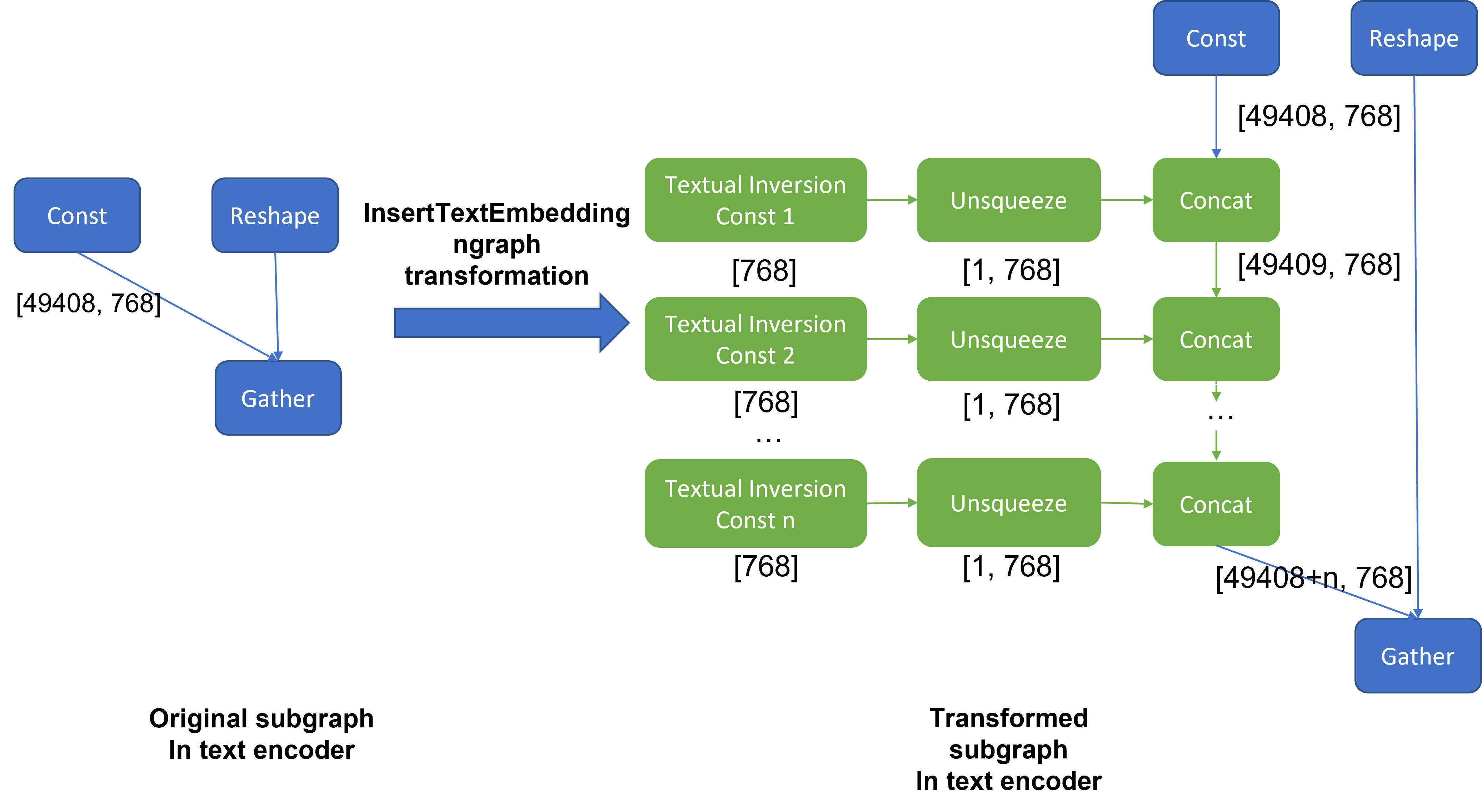
Figure 3 demonstrates the workflow of InsertTextEmbedding OpenVINOTM ngraph transformation. The left part shows the subgraph in SD 1.5 baseline text encoder model, where text embedding has a Constant node with shape [49408, 768], the 1st dimension is consistent with the original tokenizer (vocab size 49408), and the second dimension is feature length of each text embedding.
When we load (multiple) textual inversion, all textual inversion embeddings will be parsed as a list of tensors with shape[768], and each textual inversion constant will be unsqueezed and concatenated with original text embeddings. The right part is the result of applying InsertTextEmbedding ngraph transformation on the original text encoder, the green rectangle represents merged textual inversion subgraph.
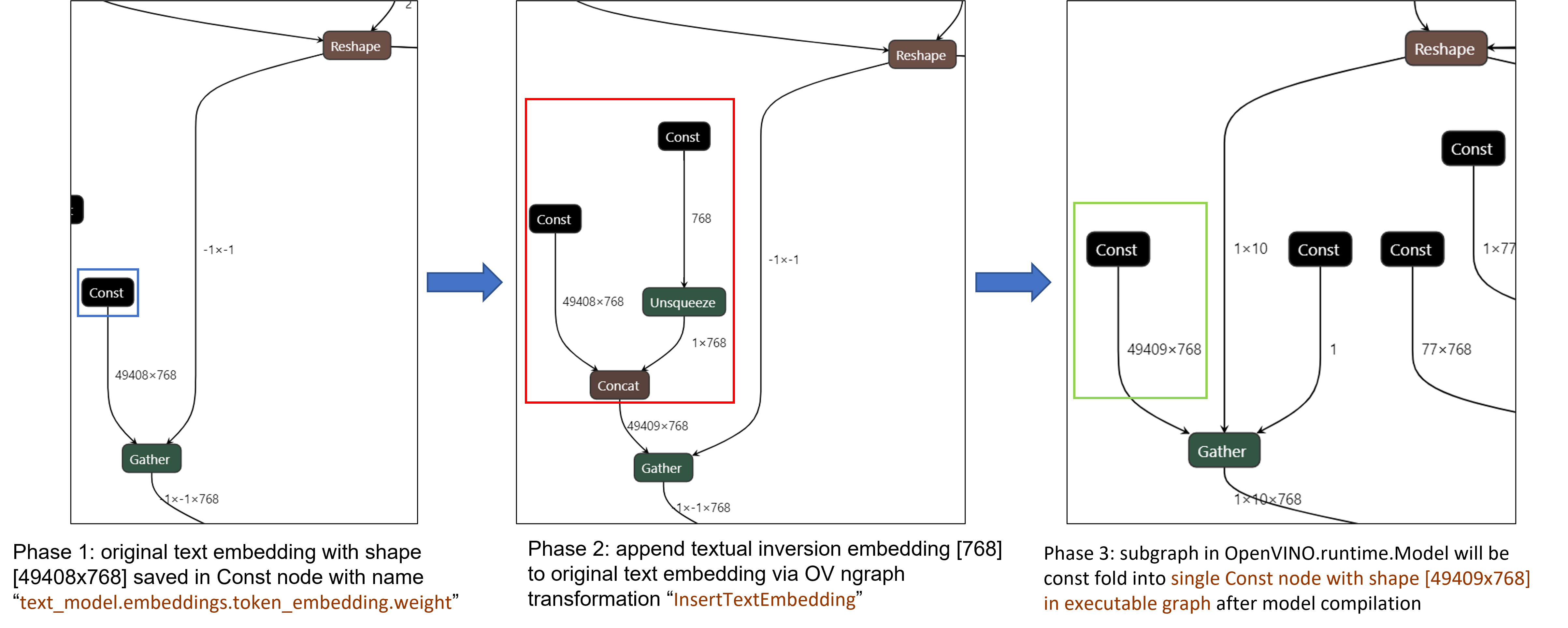
As Figure 4 shows, In the first phase, the original text embedding (marked as blue rectangle) is saved in Const node “text_model.embeddings.token_embedding.weight” with shape [49408,768], after InsertTextEmbedding ngraph transformation, new subgraph (marked as red rectangle) will be created in 2nd phase. In the 3rd phase, during model compilation, the new subgraph will be const folding into a single const node (marked as green rectangle) with a new shape [49409,768] by OpenVINOTM ConstantFolding transformation.
Stable Diffusion Textual Inversion Sample
Here are textual inversion examples verified with Stable Diffusion v1.5, Stable Diffusion v2.1 and Stable Diffusion XL 1.0 Base pipeline with latest optimum-intel
Setup Environment
Run SD 1.5 + Cat-Toy Textual Inversion Example

Run SD 2.1 + Midjourney 2.0 Textual Inversion Example

Run SDXL 1.0 Base + CharTurnerV2 Textual Inversion Example

Conclusion
In this blog, we proposed to load textual inversion embedding in the stable diffusion pipeline in runtime to save disk storage while keeping flexibility.
- Implemented OVTextualInversionLoaderMixin to update tokenizer with additional token id and update text encoder with InsertTextEmbedding OpenVNO ngraph transformation.
- Provides sample code to load textual inversion with SD 1.5, SD 2.1, and SDXL 1.0 Base and inference with Optimum-Intel
Reference
An Image is Worth One Word: Personalizing Text-to-Image Generation using Textual Inversion
Enable LoRA weights with Stable Diffusion Controlnet Pipeline
Authors: Zhen Zhao(Fiona), Kunda Xu
Low-Rank Adaptation(LoRA) is a novel technique introduced to deal with the problem of fine-tuning Diffusers and Large Language Models (LLMs). In the case of Stable Diffusion fine-tuning, LoRA can be applied to the cross-attention layers for the image representations with the latent described. You can refer HuggingFace diffusers to understand the basic concept and method for model fine-tuning: https://huggingface.co/docs/diffusers/training/lora
In this blog, we aimed to introduce the method building up the pipeline for Stable Diffusion + ControlNet with OpenVINO™ optimization, and enable LoRA weights for Unet model of Stable Diffusion to generate images with different styles. The demo source code is based on: https://github.com/FionaZZ92/OpenVINO_sample/tree/master/SD_controlnet
Stable Diffusion ControlNet Pipeline
Step 1: Environment preparation
First, please follow below method to prepare your development environment, you can choose download model from HuggingFace for better runtime experience. In this case, we choose controlNet for canny image task.
* Please note, the diffusers start to use `torch.nn.functional.scaled_dot_product_attention` if your installed torch version is >= 2.0, and the ONNX does not support op conversion for “Aten:: scaled_dot_product_attention”. To avoid the error during the model conversion by “torch.onnx.export”, please make sure you are using torch==1.13.1.
Step 2: Model Conversion
The demo provides two programs, to convert model to OpenVINO™ IR, you should use “get_model.py”. Please check the options of this script by:
In this case, let us choose multiple batch size to generate multiple images. The common application of vison generation has two concepts of batch:
- `batch_size`: Specify the length of input prompt or negative prompt. This method is used for generating N images with N prompts.
- `num_images_per_prompt`: Specify the number of images that each prompt generates. This method is used to generate M images with 1 prompts.
Thus, for common user application, you can well use these two attributes in diffusers to generate N*M images by N prompts with increased random seed values. For example, if your basic seed is 42, to generate N(2)*M(2) images, the actual generation is like below:
- N=1, M=1: prompt_list[0], seed=42
- N=1, M=2: prompt_list[0], seed=43
- N=2, M=1: prompt_list[1], seed=42
- N=2, M=2: prompt_list[1], seed=43
In this case, let’s use N=2, M=1 as a quick example for demonstration, thus the use`--batch 2`. This script will generate static shape model by default. If you are using different value of N and M, please specify `--dynamic`.
Please check your current path, make sure you already generated below models currently. Other ONNX files can be deleted for saving space.
- controlnet-canny.<xml|bin>
- text_encoder.<xml|bin>
- unet_controlnet.<xml|bin>
- vae_decoder.<xml|bin>
* If your local path already exists ONNX or IR model, the script will jump tore-generate ONNX/IR. If you updated the pytorch model or want to generate model with different shape, please remember to delete existed ONNX and IR models.
Step 3: Runtime pipeline test
The provided demo program `run_pipe.py` is manually build-up the pipeline for StableDiffusionControlNet which refers to the original source of `diffusers.StableDiffusionControlNetPipeline`
The difference is we simplify the pipeline with 4 models’ inference by OpenVINO™ runtime API which can make sure the model inference can be accelerated on Intel® CPU and GPU platform.
The default iteration is 20, image shape is 512*512, seed is 42, and the input image and prompt is for “Girl with Pearl Earring”. You can adjust or custom your own pipeline attributes for testing.
In the case with batch_size=2, the generated image is like below:

Enable LoRA weights for Stable Diffusion
Normal LoRA weights has two types, one is ` pytorch_lora_weights.bin`,the other is using safetensors. In this case, we introduce both methods for these two LoRA weights.
The main idea for LoRA weights enabling, is to append weights onto the original Unet model of Stable Diffusion, then export IR model of Unet which remains LoRA weights.
There are various LoRA models on https://civitai.com/tag/lora , we choose some public models on HuggingFace as an example, you can consider toreplace with your owns.
Step 4-1: Enable LoRA by pytorch_lora_weights.bin
This step introduces the method to add lora weights to Unet model of Stable Diffusion by `pipe.unet.load_attn_procs(...)` function. By using this way, the LoRA weights will be loaded into the attention layers of Unet model of Stable Diffusion.
* Remember to delete exist Unet model to generate the new IR with LoRA weights.
Then, run pipeline inference program to check results.
The LoRA weights appended Stable Diffusion model with controlNet pipeline can generate image like below:

Step 4-2: Enable LoRA by safetensors typed weights
This step introduces the method to add LoRA weights to Stable diffusion Unet model by `diffusers/scripts/convert_lora_safetensor_to_diffusers.py`. Diffusers provide the script to generate new Stable Diffusion model by enabling safetensors typed LoRA model. By this method, you will need to replace the weight path to new generated Stable Diffusion model with LoRA. You can adjust value of `alpha` option to change the merging ratio in `W = W0 + alpha * deltaW` for attention layers.
Then, run pipeline inference program to check results.
The LoRA weights appended SD model with controlnet pipeline can generate image like below:

Step 4-3: Enable runtime LoRA merging by MatcherPass
This step introduces the method to add lora weights in runtime before Unet or text_encoder model compiling. It will be helpful to client application usage with multiple different LoRA weights to change the image style by reusing the same Unet/text_encoder structure.
This method is to extract lora weights in safetensors file and find the corresponding weights in Unet model and insert lora weights bias. The common method to add lora weights is like:
W = W0 + W_bias(alpha * torch.mm(lora_up, lora_down))
I intend to insert Add operation for Unet's attentions' weights by OpenVINO™ `opset10.add(W0,W_bias)`. The original attention weights in Unet model is loaded by `Const` op, the common processing path is `Const->Convert->Matmul->...`, if we add the lora weights, we should insert the calculated lora weight bias as `Const->Convert->Add->Matmul->...`. In this function, we adopt `openvino.runtime.passes.MatcherPass` to insert `opset10.add()` with call_back() function iteratively.
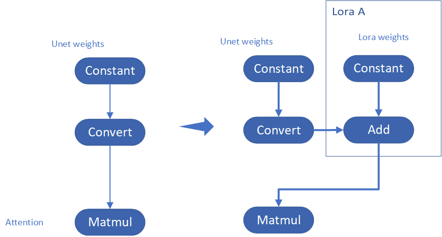
Your own transformation operations will insert opset.Add() firstly, then during the model compiling with device. The graph will do constant folding to combine the Add operation with following MatMul operation to optimize the model runtime inference. Thus, this is an effective method to merge LoRA weights onto original model.
You can check with the implementation source code, and find out the definition of the MatcherPass function called `InsertLoRA(MatcherPass)`:
The `InsertLoRA(MatcherPass)` function will be registered by `manager.register_pass(InsertLoRA(lora_dict_list))`, and invoked by `manager.run_passes(ov_unet)`. After this runtime MatcherPass operation, the graph compile with device plugin and ready for inference.
Run pipeline inference program to check the results. The result is same as Step 4-2.
The LoRA weights appended Stable Diffusion model with controlNet pipeline can generate image like below:

Step 4-4: Enable multiple LoRA weights
There are many different methods to add multiple LoRA weights. I list two methods here. Assume you have two LoRA weigths, LoRA A and LoRA B. You can simply follow the Step 4-3 to loop the MatcherPass function to insert between original Unet Convert layer and Add layer of LoRA A. It's easy to implement. However, it is not good at performance.
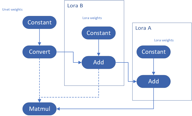
Please consider about the Logic of MatcherPass function. This fucntion required to filter out all layer with the Convert type, then through the condition judgement if each Convert layer connected by weights Constant has been fine-tuned and updated in LoRA weights file. The main costs of LoRA enabling is costed by InsertLoRA() function, thus the main idea is to just invoke InsertLoRA() function once, but append multiple LoRA files' weights.
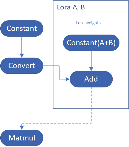
By above method to add multiple LoRA, the cost of appending 2 or more LoRA weights almost same as adding 1 LoRA weigths.
Now, let's change the Stable Diffusion with dreamlike-anime-1.0 to generate image with styles of animation. I pick two LoRA weights for SD 1.5 from https://civitai.com/tag/lora.
- soulcard: https://civitai.com/models/67927?modelVersionId=72591
- epi_noiseoffset: https://civitai.com/models/13941/epinoiseoffset
You probably need to do prompt engineering work to generate a useful prompt like below:
- prompt: "1girl, cute, beautiful face, portrait, cloudy mountain, outdoors, trees, rock, river, (soul card:1.2), highly intricate details, realistic light, trending on cgsociety,neon details, ultra realistic details, global illumination, shadows, octane render, 8k, ultra sharp"
- Negative prompt: "3d, cartoon, lowres, bad anatomy, bad hands, text, error"
- Seed: 0
- num_steps: 30
- canny low_threshold: 100
You can get a wonderful image which generate an animated girl with soulcard typical border like below:

Additional Resources
Provide Feedback & Report Issues
Notices & Disclaimers
Intel technologies may require enabled hardware, software, or service activation.
No product or component can be absolutely secure.
Your costs and results may vary.
Intel does not control or audit third-party data. You should consult other sources to evaluate accuracy.
Intel disclaims all express and implied warranties, including without limitation, the implied warranties of merchantability, fitness for a particular purpose, and non-infringement, as well as any warranty arising from course of performance, course of dealing, or usage in trade.
No license (express or implied, by estoppel or otherwise) to any intellectual property rights is granted by this document.
© Intel Corporation. Intel, the Intel logo, and other Intel marks are trademarks of Intel Corporation or its subsidiaries. Other names and brands may be claimed as the property of others.
Accelerate DIEN for Click-Through-Rate Prediction with OpenVINO™
Author: Xiake Sun, Cecilia Peng
Introduction
A click-through rate (CTR) prediction model is designed to estimate how likely a user will click on an advertisement or item. Deployment of a CTR model is considered one of the core tasks in e-commerce, as its performance not only affects platform revenue but also influences customers’ online shopping experience.
Deep Interest Evolution Network (DIEN) developed by Alibaba Group aims to better predict customer’s CTR to improve the effectiveness of advertisement display. DIEN proposes the following two modules:
- Temporally captures and extracts latent interests based on customer history behaviors.
- Models an evolving process of user interests using GRU with an attentional update gate (AUGRU)
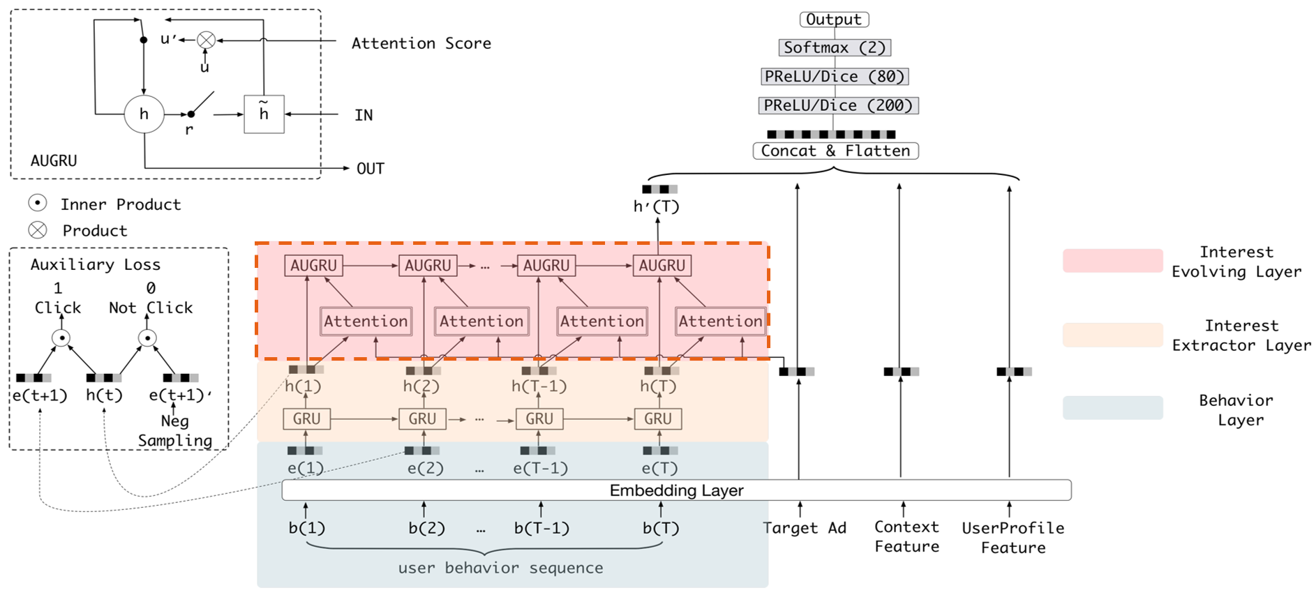
Figure 1 shows the structure of DIEN, with the help of AUGRU, DIEN can overcome the disturbance from interest drifting, which improves the performance of CTR prediction largely in online advertising system.
DIEN Optimization with OpenVINOTM
Here we introduce DIEN optimization with OpenVINOTM in two aspects: graph level and dynamism runtime optimization.
Graph Level Optimization
Figure 2 shows the AUGRU subgraph of DIEN visualized in Netron.
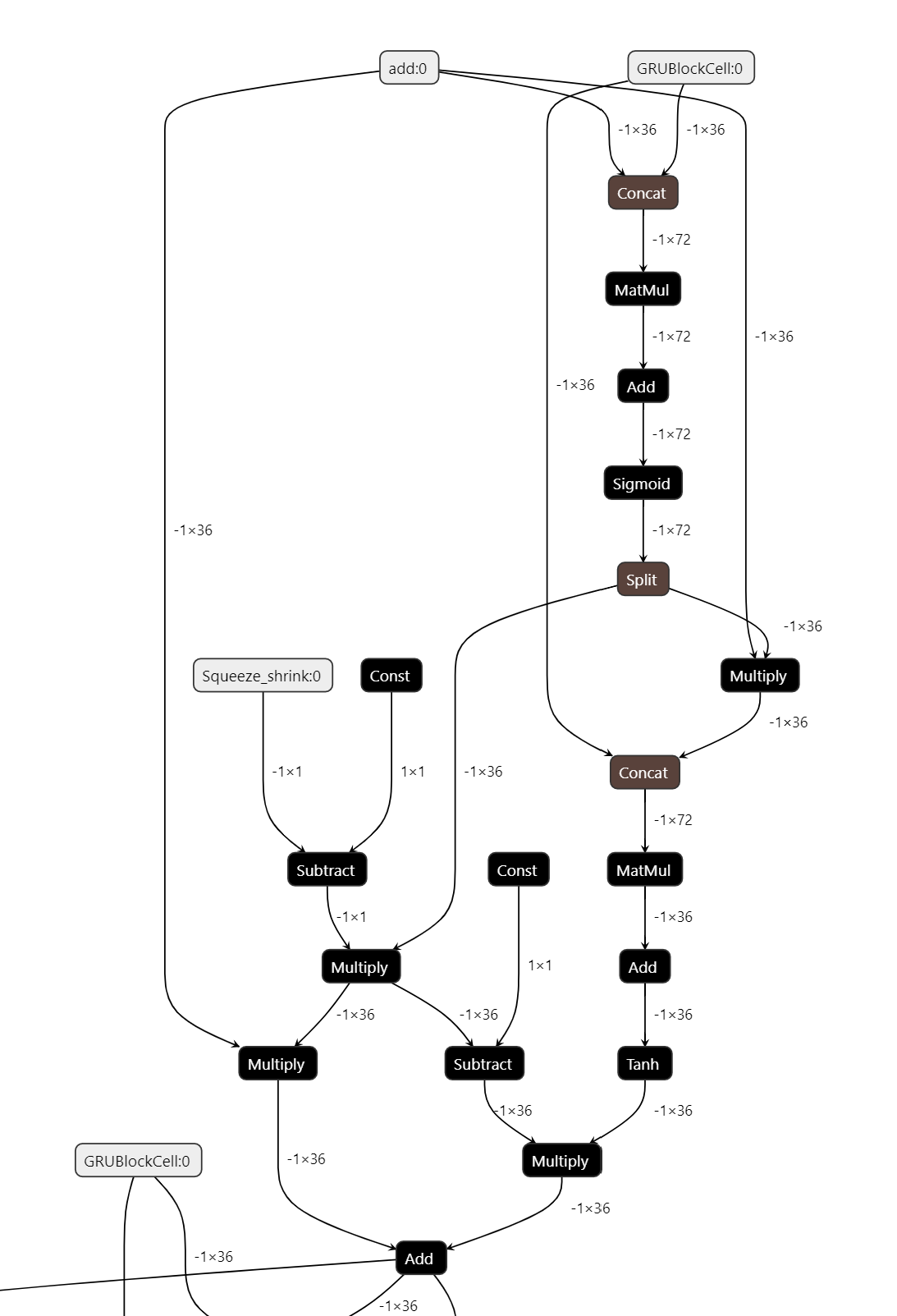
OpenVINOTM implements internal operations AUGRUCell and AUGRUSequence for better graph-level optimization. Each decomposed subgraph of GRU and AUGRU is fused into a corresponding cell operator respectively. What's more, in case of static sequence length, the group of consecutive cells are further fused into a sequence operator. In case of dynamic sequence length, however, the sequence is processed with a loop of cells due to the limitation of oneDNN RNN primitive. This loop of cells is TensorIterator and (AU)GRUCell. We will introduce the optimizations of TensorIterator in next session.
TensorIterator Runtime Optimization with Dynamic Shape
Before we dive into optimization details, let’s first checkout how OpenVINOTM TensorIterator operation works.
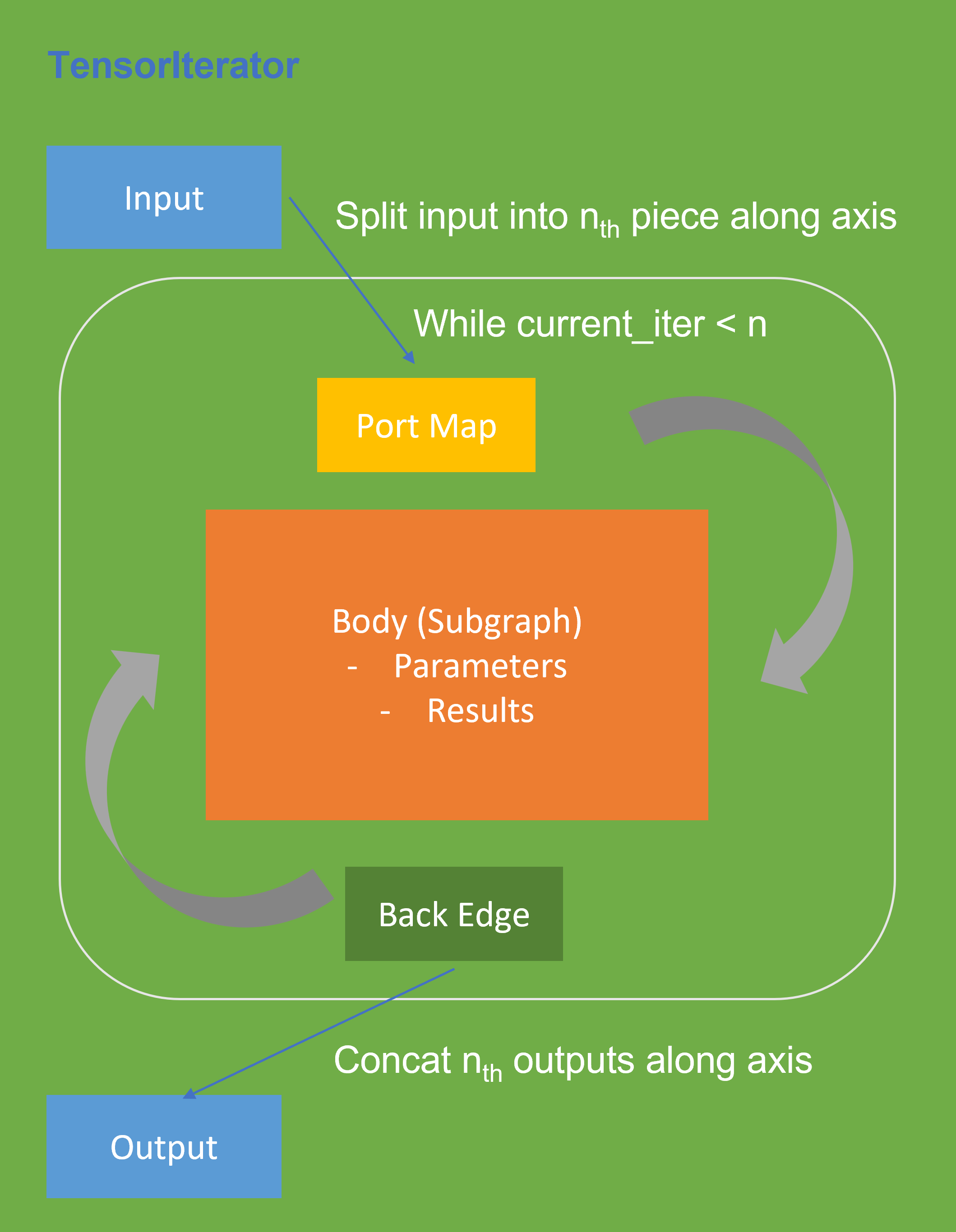
The TensorIterator layer performs recurrent execution of thenetwork, which is described in the body, iterating through the data. Figure 3 shows the workflow of OpenVINOTM Operation TensorIterator in a simplified view. For details, please refer to the specification.
Similar to other layers, TensorIterator has regular sections: input and output. It allows connecting TensorIterator to the rest of the IR. TensorIterator also has several special sections: body, port_map, back_edges. The principles of their work are described below.
- body is a network that will be recurrently executed. The network is described layer by layer as a typical IR network.
- port_map is a set of rules to map input or output data tensors of TensorIterator layer onto body data tensors. The port_map entries can be input and output. Each entry describes a corresponding mapping rule.
- back_edges is a set of rules to transfer tensor values from body outputs at one iteration to body parameters at the next iteration. Back edge connects some Result layers in body to Parameter layer in the same body.
If output entry in the Port map doesn’t have partitioning (axis, begin, end, strides) attributes, then the final value of output of TensorIterator is the value of Result node from the last iteration. Otherwise, the final value of output of TensorIterator is a concatenation of tensors in the Result node for all body iterations.
We use Intel® VTune™ Profiler to run benchmark_app with DIEN FP32 IR model on Intel® Xeon® Gold 6252N Processor for performance profiling.
Cache internal reorder primitives in TensorIterator
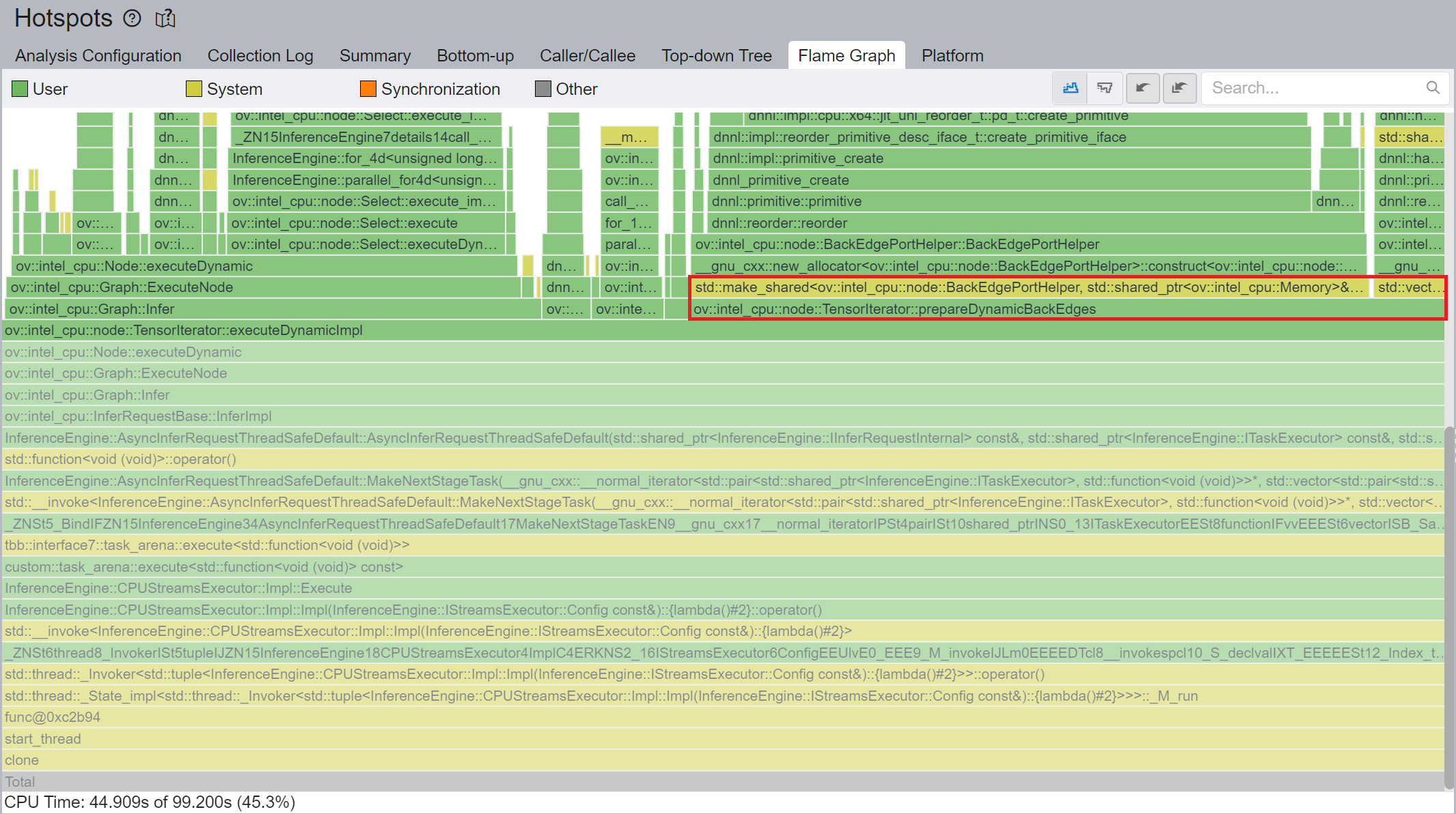
Figure 4 shows that TensorIterator::prepareDynamicBackEdges() spends nearly 45% CPU time to create the reorder primitives. DIEN FP32 model has 2 TensorIterator, eachTensorIterator runs 100 iterations in body with the same input/output shape regarding the current batch. Besides, each TensorIterator has 7 back edges, which means the reorder primitive are frequently created.
So, we propose to cache internal reorder primitive in TensorIterator to optimize back edge memory copy logic. With this optimization, the performance with dynamic shape can be improved by 8x times.
Memory allocation and reuse optimization in TensorIterator
As Figure 3 shows, if we have split input as nth piece to loop in body, at the end, the outputs of TensorIterator will be a concatenation of tensors in the Result node for all body iterations, which can lead to performance overhead. Based on previous optimization we re-run performance profiling using benchmark_app with DIEN FP32 IR model on Intel® Xeon® Gold 6252N Processor as showed in Figure 5.
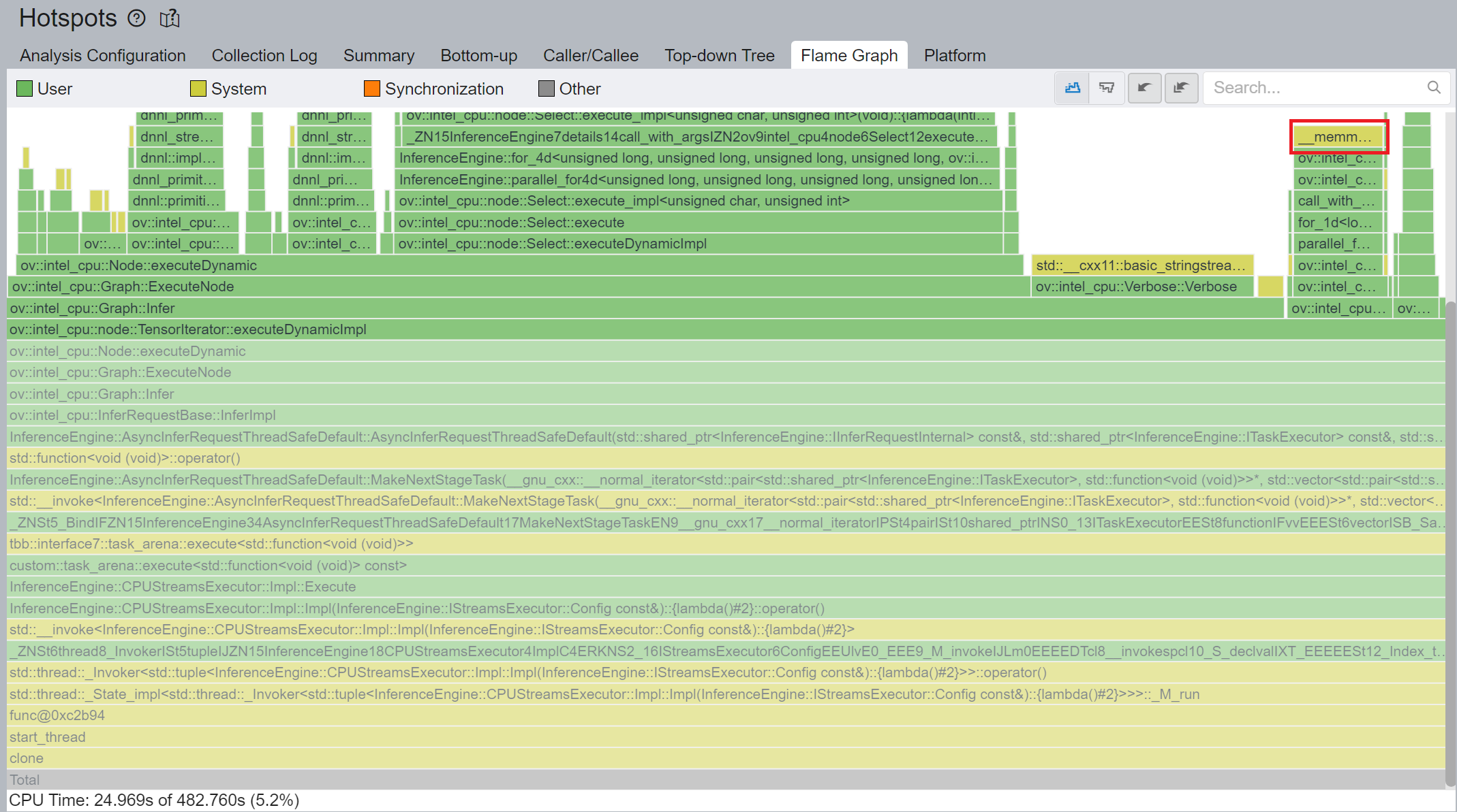
CPU plugin TensorIterator supports both two operators - TensorIterator and Loop. The outputs of each iteration could be concatenated and return to users. Since the output size is not always known before the execution, the legacy implementation is to dynamically allocate the concatenated output buffer.
We propose two points from the memory allocation standpoint:
- In the case of TensorIterator number of iterations is determined by the size of the axis we are slicing. So, if TensorIterator body one ach iteration will produce the same shape on output we can easily preallocate enough memory before the TI computation, The same for Loop with trip count input - we can just read the value from this input, make shape inference for the body and this determines the required amount of memory.
- More complicated story is when we don't know exact number of iterations before Loop inference (e.g., number of iterations is determined by ExecutionCondition input). In that case do the following: let’s have an output buffer where we put the Loop output. Once the buffer doesn't have enough space, we reallocate it on new size based on a simple and effective dynamic array algorithm.
OpenVINOTM implemented memory allocation and reuse optimization in TensorIterator to significantly reduce the number of reallocations and not to allocate to much memory at the same time. Experiments show that performance can be further improved by more than 20%.
DIEN OpenVINOTM Demo
Clone demo repository:
Prepare Amazon dataset:
Setup Python Environment:
Convert original TensorFlow model to OpenVINOTM FP32 IR:
Run the Benchmark with TensorFlow backend:
Run the Benchmark with OpenVINOTM backend using FP32 inference precision:
Run the Benchmark with OpenVINOTM backend using BF16 inference precision:
Please note, Xeon native supports BF16 infer precision since 4th Generation Intel® Xeon® Scalable Processors. Running BF16 on a legacy Xeon platform may lead to performance degradation.
Conclusion
In this blog, we introduce inference optimization of DIEN recommendation model with OpenVINOTM runtime as follows:
- For static input sequence length, AUGRU subgraph will be decomposed and fused as AUGRU and AUGRUSequence OpenVINOTM internal operation.
- For dynamic input sequence length, we propose cache internal reorder primitives and memory allocation and re-use optimization in TensorIterator.
- Provide a demo for model enabling and efficient inference of DIEN with OpenVINOTM runtime.
Reference
Deep Interest Evolution Network (DIEN)
Encrypt Your Dataset and Train Your Model with It Directly
Encrypt Your Dataset and Train Your Model with It Directly

Introduction
When we deal with dataset for creating AI models, we need to consider sensitive information managed and stored online in the cloud or on connected devices. Unsecured datasets can be vulnerable to unauthorized access, theft, and misuse, particularly when processed for machine learning workloads. Certain fields, such as industrial or medical sectors, face exceptionally high risks when their data is exposed to these potential threats. For example, if a dataset used to train a detection model for identifying factory process errors is leaked, it can expose sensitive factory process technology. This highlights the importance of safeguarding datasets at every stage, from data storage to model training.
Dataset Management Framework (Datumaro) offers a dataset encryption feature for AI model training. With Datumaro, you can encrypt datasets of any computer vision data format into the DatumaroBinary format. This encrypted dataset can remain encrypted as far as it is needed for decryption. By combining the encrypted dataset with OpenVINO training extensions™, you can use it directly for model training without decryption. Whenever needed, you can use Datumaro once again to decrypt the dataset and convert it back to any major computer vision data format, such as VOC, COCO, or YOLO. Please refer to another posting data_convert for data convert.
Encrypt Your Dataset Using Datumaro
Datumaro provides two ways to encrypt a dataset: CLI and Python API. First, you need to install Datumaro on your system. Please refer to the installation guide here for detailed instructions. Once you have completed the installation of Datumaro, let's first look at the CLI usage. You can encrypt a dataset using the datum convert CLI command as follows:
The necessary user inputs for this command are as follows:
- -i <input-dataset-path>: Enter the path to the dataset you want to encrypt in <input-dataset-path>.
- -o <output-dataset-path>: Enter the path where the encrypted dataset will be produced in <output-dataset-path>.
NOTE:: (Optional) You can additionally specify the data format of your input dataset by entering the -if <input-dataset-format> argument. In most cases, Datumaro can automatically infer the data format of the input dataset, but it might fail. In such cases, you can use the datum detect --show-rejections <input-dataset-path> command to identify the cause of the failure while inferring the data format.
NOTE:: The --save-media argument is a flag that allows you to convert your media files (e.g., images) as well. If this argument is not provided, the encrypted media will not be included in the output directory and only the encrypted annotations are included in the output directory.
Next, let's take a look at how to encrypt a dataset using the Python API. Please examine the following code snippet:
You import the dataset by specifying the path of the input dataset in the import_from function as path="<input-dataset-path>". Then, to export the dataset, you specify the path of the output dataset in the save_dir="<output-dataset-path>" of the export function. Similarly, you also need to provide the encryption=True and format="datumaro_binary" keyword arguments as in the CLI example. A more detailed end-to-end example for this can be found in a Jupyter notebook. Please refer to this link for more information.
So far, all the examples have used the datumaro_binary (DatumaroBinary) format for the exported dataset. Currently, the dataset encryption feature is only supported for the datumaro_binary format. DatumaroBinary is a Datumaro's own data format that stores annotation data in binary representation. It is much faster and storage efficient compared to string-based datasets such as COCO based on JSON. For more detailed information about DatumaroBinary, please refer to this link.
How Datumaro Encrypts Your Dataset?
Datumaro uses the Fernet symmetric encryption recipe provided by the cryptography library to encrypt the dataset. Fernet is built on top of a number of standard cryptographic primitives such as AES or HMAC, and hence Fernet guarantees that a message encrypted cannot be manipulated or read without the key. Please refer to this link for detailed information.
When encrypting the dataset, Datumaro generates a secret key through Fernet and saves it as a txt file at the following path: <output-dataset-path>/secret_key.txt. The secret key generated at this path is a 50-characters string, which consists of a randomly generated 32-bytes string encoded in base64, with the prefix datum- added.
If you have checked the secret key in this file, you must ensure that it is not in the same location with the dataset. If this secret key is uncovered, an attacker would be able to access the contents of the encrypted dataset. Additionally, this secret key is required when training models using OpenVINO training extensions™ with the encrypted dataset or when decrypting it later. Therefore, you should be careful not to lose this secret key.
The following table briefly shows how the data is encrypted. The binary representation of the data is encrypted, so that the following image cannot be seen by the image viewer.
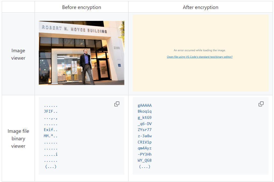
Train Your Model with the Encrypted Dataset Using OpenVINO Training Extensions™
OpenVINO training extensions™ is a tool that allows convenient training of computer vision models and accelerated inference on Intel® devices by exporting trained models to OpenVINO Intermediate Representation (IR) through a CLI. Within the OpenVINO ecosystem, Datumaro is integrated with OpenVINO training extensions™ as a dataset interface. Therefore, the encrypted dataset can be directly used for model training through OpenVINO training extensions™. For detailed installation instructions of OpenVINO training extensions™, please refer to the following link.
Next, let's explore how to use the encrypted dataset directly for model training through the CLI command.
The user inputs required for this command are as follows:
- --train-data-roots <encrypted-dataset-path> and --val-data-roots <encrypted-dataset-path>: Specify the path to the encrypted dataset by replacing <encrypted-dataset-path>. Since the DatumaroBinary format uses the same root directory for both the training and validation subsets, both arguments should have the same value.
- --encryption-key <secret-key>: Provide the secret key corresponding to the encrypted dataset in <secret-key>. This is the 50-character string with the datum- prefix described in the previous section.
NOTE:: <template> is the name of the model template provided by OpenVINO training extensions™. A model template is a recipe for a deep learning model for a specific computer vision task. To explore all the model templates supported by OpenVINO training extensions™, you can use the otx find CLI command or refer to this link.
Decrypt the Encrypted Dataset Using Datumaro
If you want to utilize the encrypted dataset in another AI workload, you need to decrypt the encrypted data. This process reverses the dataset encryption using Datumaro, and encryption-decryption preserves all the information without loss. Similar to the previous section, decryption can be done using the CLI or Python API. Let's first look at decryption using the CLI.
You can use the same datum convert command as before. However, specify the path to the encrypted dataset as the input dataset path (-i <encrypted-dataset-path>), and provide the secret key, which is a 50-character string with the datum- prefix described in the previous section, as the <secret-key> argument for --encryption-key <secret-key>. Additionally, you can choose any data format supported by Datumaro as the output data format. To learn more about the data formats supported by Datumaro, refer to this link.
Next, let's see how decryption can be done using Python API.
Similar to the CLI method, provide the path to the encrypted dataset and the secret key as arguments to the import_from function. For the export function, specify the output dataset path and the output data format.
Conclusion
This post introduced dataset encryption feature provided by Datumaro. It demonstrated how to encrypt a dataset using Datumaro and train a model with the encrypted dataset using OpenVINO training extensions™. Whenever needed you can decrypt it with Datumaro for other AI projects and training frameworks. You can refer to the end-to-end Jupyter notebook example provided on this blog post here for step-by-step guide. The features introduced in this post are available in Datumaro version 1.4.0 or higher and OpenVINO training extensions™ version 1.4.0 or higher.
Datumaro offers a range of useful features for managing datasets besides the dataset encryption feature. You can find examples of other Datumaro features, such as noisy label detection during training with OpenVINO training extensions™, in the Jupyter examples directory. For more information about Datumaro and its capabilities, you can visit the Datumaro documentation page. If you have any questions or requests about using Datumaro, feel free to open an issue here.

