

OpenVINO Blog

OpenVINO™ Enable PaddlePaddle Quantized Model
OpenVINO™ is a toolkit that enables developers to deploy pre-trained deep learning models through a C++ or Python inference engine API. The latest OpenVINO™ has enabled the PaddlePaddle quantized model, which helps accelerate their deployment.
From floating-point model to quantized model in PaddlePaddle
Baidu releases a toolkit for PaddlePaddle model compression, named PaddleSlim. The quantization is a technique in PaddleSlim, which reduces redundancy by reducing full precision data to a fixed number so as to reduce model calculation complexity and improve model inference performance. To achieve quantization, PaddleSlim takes the following steps.
- Insert the quantize_linear and dequantize_linear nodes into the floating-point model.
- Calculate the scale and zero_point in each layer during the calibration process.
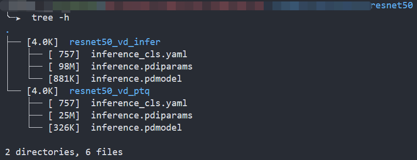
- Convert and export the floating-point model to quantized model according to the quantization parameters.
As the Figure1 shows, Compared to the floating-point model, the size of the quantized model is reduced by about 75%.
Enable PaddlePaddle quantized model in OpenVINO™
As the Figure2.1 shows, paired quantize_linear and dequantize_linear nodes appear intermittently in the model.
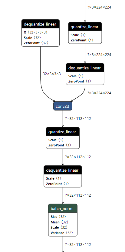
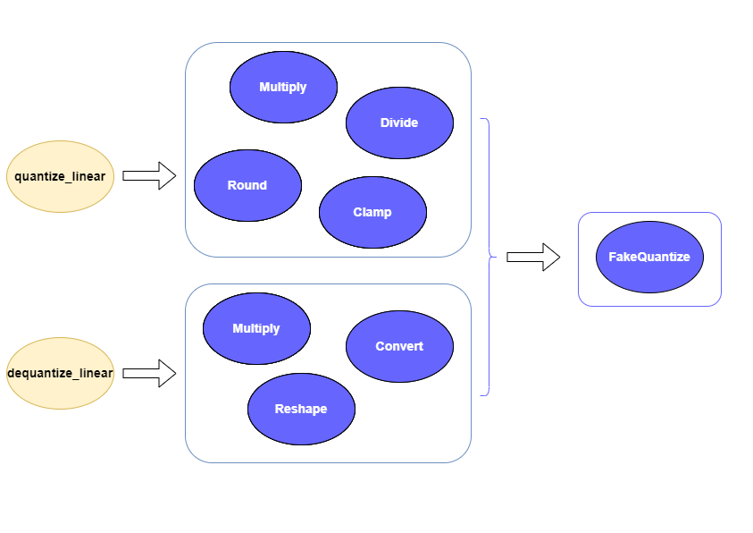
In order to enable PaddlePaddle quantized model, both quantize_linear and dequantize_linear nodes should be mapped first. And then, quantize_linear and dequantize_linear pattern scan be fused into FakeQuantize nodes and OpenVINO™ transformation mechanism will simplify and optimize the model graph in the quantization mode.
To check the kernel execution function, just profile and dump the execution progress, you can use benchmark_app as an example. The benchmark_app provides the option"-pc", which is used to report the performance counters information.
- To report the performance counters information of PaddlePaddle resnet50 float model, we can run the command line:
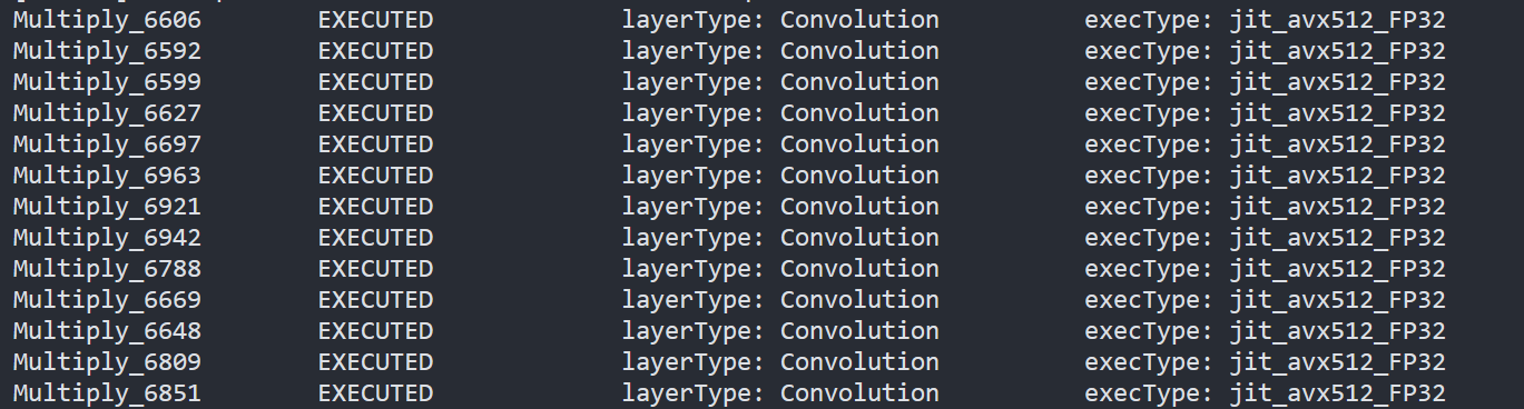
- To report the performance counters information of PaddlePaddle resnet50 quantized model, we can run the command line:
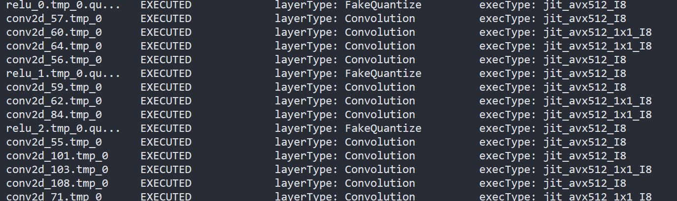
By comparing the Figure2.3 and Figure2.4, we can easily find that the hotpot layers of PaddlePaddle quantized model are dispatched to integer ISA implementation, which can accelerate the execution.
Accuracy
We compare the accuracy between resnet50 floating-point model and post training quantization(PaddleSlim PTQ) model. The accuracy of PaddlePaddle quantized model only decreases slightly, which is expected.
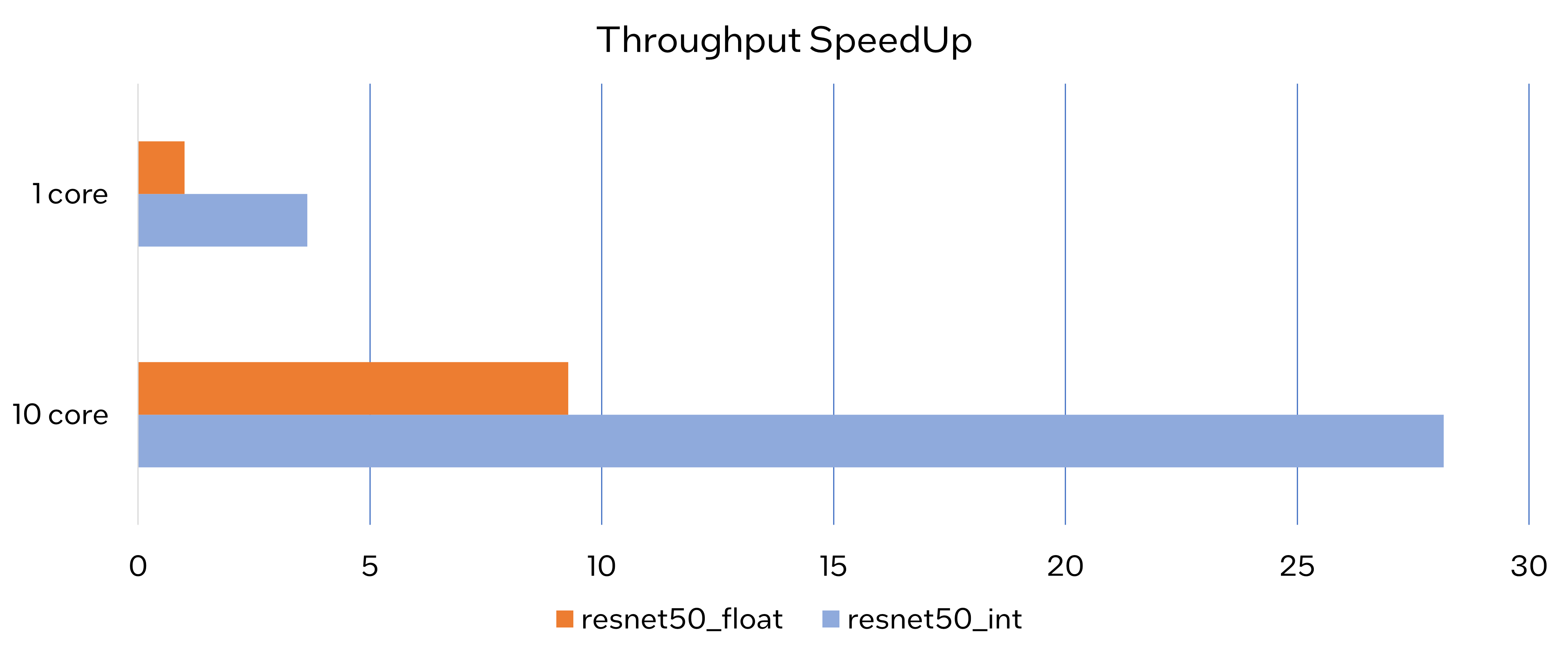
Performance
Throughput Speedup
The throughput of PaddlePaddle quantized resnet50 model can improve >3x.
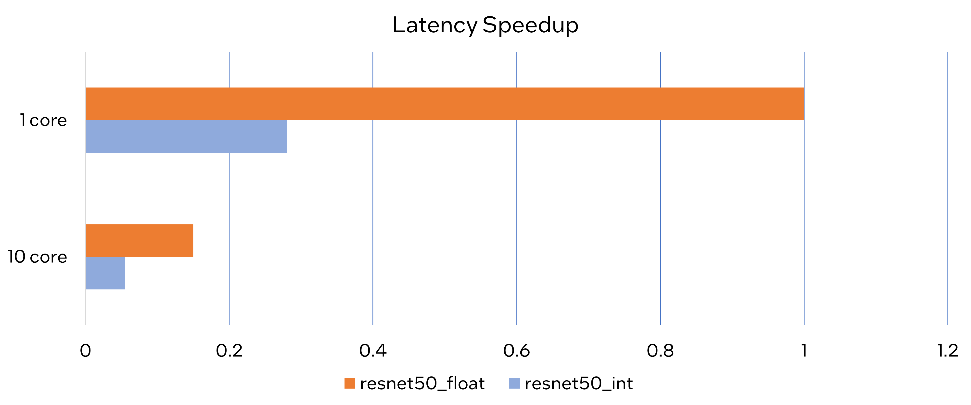
Latency Speedup
The latency of PaddlePaddle quantized resnet50 model can reduce about 70%.
Conclusion
In this article, we elaborated the PaddlePaddle quantized model in OpenVINO™ and profiled the accuracy and performance. By enabling the PaddlePaddle quantized model in OpenVINO™, customers can accelerate both throughput and latency of deployment easily.
Notices & Disclaimers
- The accuracy data is collected based on 50000 images of val dataset in ILSVRC2012.
- The throughput performance data is collected by benchmark_app with data_shape "[1,3,224,224]" and hint throughput.
- The latency performance data is collected by benchmark_app with data_shape "[1,3,224,224]" and hint latency.
- The machine is Intel® Xeon® Gold 6346 CPU @3.10GHz.
- PaddlePaddle quantized model can be achieve at https://github.com/PaddlePaddle/FastDeploy/blob/develop/docs/en/quantize.md.
Benchmark_app Servers Usage Tips with Low-level Setting for CPU
We provide tips for Benchmark_app in different situations like VPS and bare metal servers. The tips aim at practical evaluation with limited hardware resources. Help customers quickly balance performance and hardware resource requirements when deploying AI on servers. Besides the suggestion of different level settings on devices, the tables of evaluation would help in the analysis and verification.
The benchmark app provides various options for configuring execution parameters. For instance, the benchmark app allows users to provide high-level “performance hints” for setting latency-focused or throughput-focused inference modes. The official online documentation provides a detailed introduction from a technical perspective. To further reduce learning costs, this blog provides guidance for actual deployment scenarios for customers. Besides the high-level hints, the low-level setting as the number of streams will be discussed with the numactl on the CPU.
Benchmark_app Tips for CPU On VPS
Tip 1: For initial model testing, it is recommended to use the high-level settings of Python version Benchmark_app without numactl directly.
Python version Benchmark_app Tool:
In this case, the user is mainly testing the feasibility of the model. The Python benchmark_app is recommended for fast testing, for it is automatically installed when you install OpenVINO Developer Tools using PyPI. The Benchmark C++ Tool needs to be built following the Build the Sample Applications instructions.
For basic usage, the basic configuration options like “-m” PATH_TO_MODEL, “-d” TARGET_DEVICE are enough. If further debugging is required, all configuration options like “-pc” are available in the official documentation.
numactl:
numactl controls the Non-uniform memory access (NUMA) policy for processes or shared memory, which is used as a global CPU control tool.
In this scenario, it is only recommended not to use numactl. Because VPS may not be able to provide real hardware information. Therefore, it is impossible to bind the CPU through numactl.
The following parts will describe how and when to use it.
High-level setting:
The preferred way to configure performance for the first time is using performance hints, for simple and quick deployment. The High-level setting means using the Performance hints“-hint” for setting latency-focused or throughput-focused inference modes. This hint causes the runtime to automatically adjust runtime parameters, such as the number of processing streams and inference batch size.
Low-level setting:
The corresponding configuration of stream and batch is the low-level setting. For the new release 22.3 LTS, Users need to disable the hints of Benchmark_app to try the low-level settings, like nstreams and nthreads.
Note:
- Could not set the device with AUTO, when setting -nstreams.
- However, in contrast to the benchmark_app, you can still combine the hints and individual low-level settings in API. For example, here is the Python code.
The low-level setting without numactl is the same on different kinds of servers. The detail will be analyzed in two parts later.
Benchmark_app Tips for CPU On Dedicated Server
Tip 2: Low-level setting without numactl, for the CPU, always use the streams first and tune with thread.
- nthreads is an integer multiple of nstreams with balancing performance and requirements.
- the Optimal Number of Inference Requests can be obtained, which can be used as a reference for further tuning.
On Dedicated Server:
Compared with VPS, the user gets full access to the hardware. It comes as a physical box, not a virtualized slice of server resources. This means no need to worry about performance drops when other users get a spike in traffic in theory. In practice, a server is shared within the group simultaneously. It is recommended to use performance hints to determine peak performance, and then tune to determine a suitable hardware resource requirement. Therefore, hardware resources (here CPU) need to be set or bound. We recommend not using numactl to control but optimizing with the low-level setting.
Low-level setting:
Stream is commonly the configurable method of this device-side parallelism. Internally, every device implements a queue, which acts as a buffer, storing the inference requests until retrieved by the device at its own pace. The devices may process multiple inference requests in parallel to improve the device utilization and overall throughput.
Unlike”-nireq”, which depends on the needs of actual scenarios, nthreads and nstreams are parameters for performance and overhead. nstreams has high priority. We will verify the conclusion with Benchmark_app. Here, we could test the different settings of the C++ version Benchmark_app with OpenVINO 22.3 LTS on a dedicated server. The C++ version is recommended for benchmarking models that will be used in C++ applications. C++ and Python tools have a similar command interface and backend.
Evaluation:-nireq -nthreads and -nstreams
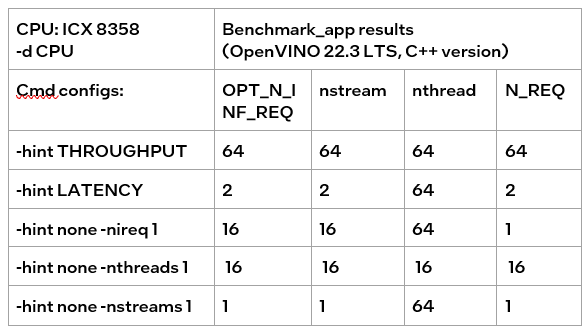
According to the results of the table, it can be obtained:
If only nireq is set, then nstreams and nthreads will be automatically set by the system according to HW. 64 threads are in the same NUMA node. CPU cores are evenly distributed between execution streams (every 4 threads). nstreams =64/4=16. For the first time, it is recommended not to set nireq. By setting other parameters of benchmark_app, the Optimal Number of Inference Requests can be obtained, which can be used as a reference for further tuning.
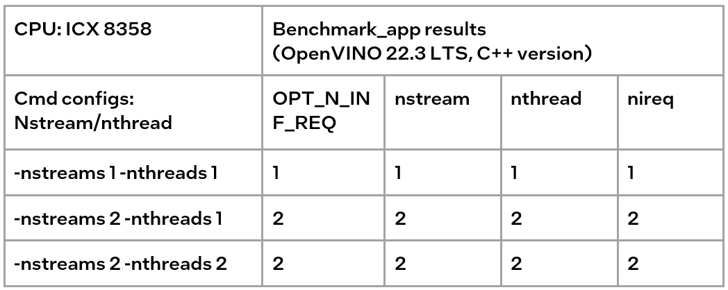
The max value of nthreads depends on the physical core. Setting nthreads alone doesn't make sense. Further tests set two of nireq, nstreams and nthreads at the same time, and the results are listed in the table below.
According to the table, when setting thread and stream simultaneously, there should be more nthreads than the nthreads. Otherwise, the default nthreads is equal to nthreads. The nthreads setting here is equivalent to binding hardware resources for the stream. This operation is implemented in the OpenVINO runtime. Users familiar with Linux may use other methods outside OpenVINO to bind hardware resources, namely numactl. As discussed before, this method is not suitable for VPS. Although not recommended, the following sections analyze the use of numactl on bare metal servers.
Tip3:
numactl is equivalent to the low-level settings on a bare metal server. Ensure the consistency of numactl and low-level settings, when using simultaneously.
The premise is to use numactl correctly, that is, use it on the same socket.
Evaluation: Low-level setting vs numactl
The numactl has been introduced above, and the usage is directly shown here.
numactl-C 0,1 . /benchmark_app -m ‘path to your model’ -hint none -nstreams 1-nthreads 1
Note:
"-C" refers to the CPUs you want to bind. You can check the numa node through “numactl–hardware”.
The actual CPU operation can be monitored through the htop tool.
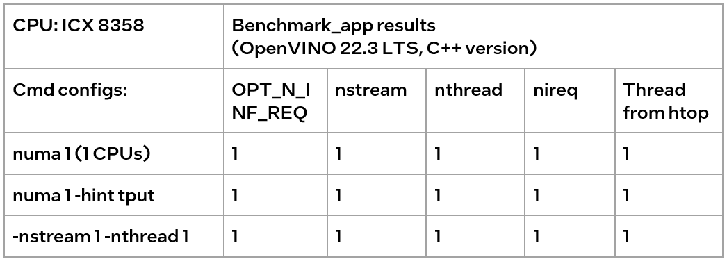
We could find out that using numactl alone or with the high-level hint is equivalent to the low-level settings. This shows that the principle of binding cores is the same. Although numactl can easily bind the core without any settings, it cannot change the ratio between nstreams and nthreads.
In addition, when numactl and the low-level setting are used simultaneously, the inconsistent settings will cause problems.
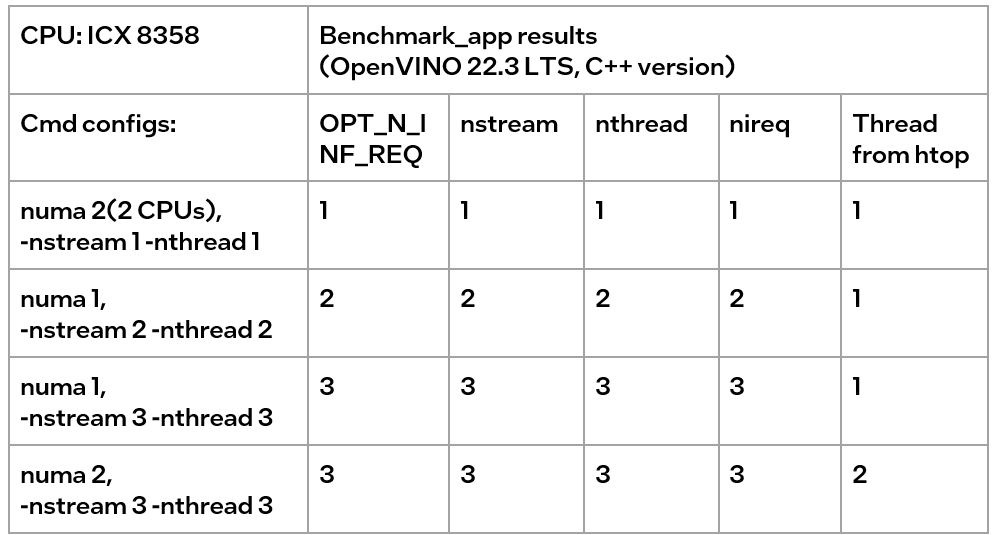
We can find the following results, according to the data in the table
- When the number of CPUs (set by NUMA) > nthread, determined by nthread, Benchmark_app results are equal to the number of CPUs monitored by htop
- When the number of CPUs (set by NUMA) < nthread, htop monitors that the number of CPUs is equal to the number controlled by NUMA, but an error message appears in Benchmark_app results, and the latency is exactly equal to the multiple of nstream.
The reason is that numactl is a global control, and benchmark_app can’t be corrected, resulting in latency equal to the result of repeated operations. The printed result is inconsistent with the actual monitoring, meaningless.
Summary:
Tip 1: For initial model testing on VPS, it is recommended to use the high-level settings of Python version Benchmark_app without numactl directly.
Tip 2: To balance the performance and hardware requirement on the bare metal server, a Low-level setting without numactl for the CPU is recommended, always set the nstreams first and tune with nthreads.
Tip 3: numactl is equivalent to the low-level settings on a bare metal server. Ensure the consistency of numactl and low-level setting, when using simultaneously.
Enable OpenVINO™ Optimization for WeNet
Introduction
The WeNet model provides two-pass approach to unify streaming and non-streaming end-to-end (E2E) speech recognition which is widely used with various HW platforms. In this blog, we provide the OpenVINO™ optimization for WeNet on Intel® platforms.
The public WeNet project is referenced from: wenet-e2e/wenet
The WeNet model can be considered as a pipeline which is split into 3 parts for decoder, CTC and encoder. Refer the model structure in below picture:
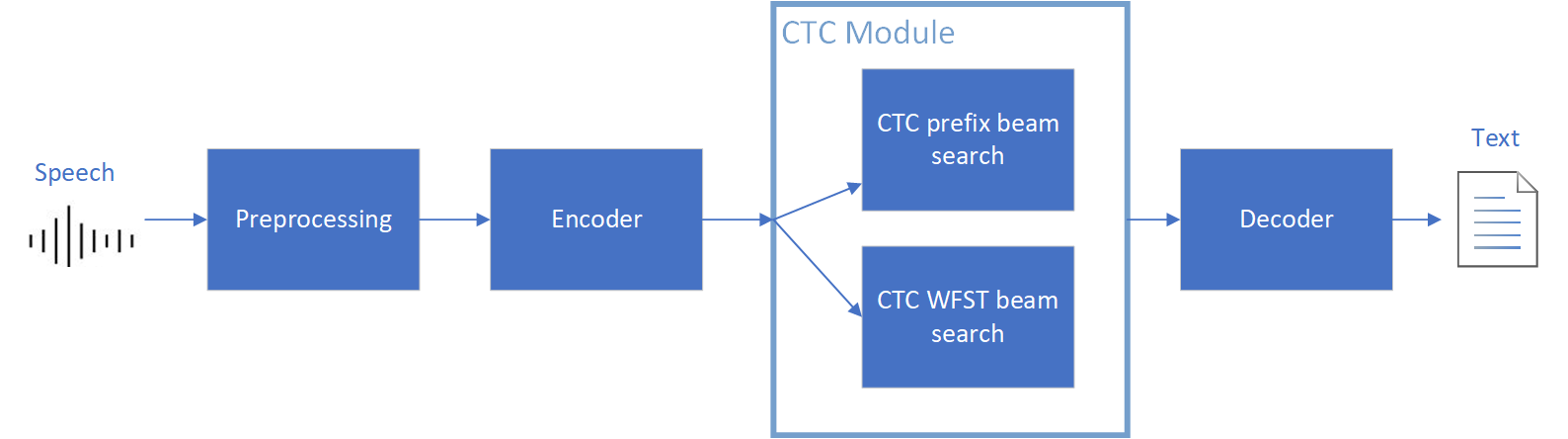
We implement the wrapper function of Automatic Speech Recognition (ASR) model class with OpenVINO™ runtime API programming for these 3 models’ data preparation and inference. Please refer the integrated OpenVINO™ optimization in official project: wenet-e2e/wenet/runtime/openvino
OpenVINO™backend on WeNet
In this project, you do not require to download OpenVINO™ and build the library with WeNet project manually. It’s already fully integrated with OpenVINO™ runtime library for downloading, program compiling and linking. If your operating system is not one of OpenVINO™ runtime library supported, the script will download OpenVINO™ source from Github, and build with CPU plugin to support.
At present, this repository already optimized and validated by OpenVINO™ 2022.3.0 version. Check the operating system which can support OpenVINO™ runtime library directly:
- Windows* 10
- CentOS 7, Red Hat* Enterprise Linux* 8
- Ubuntu* 18.04, 20.04
- Debian 9.13 for X86
- macOS* 10.15
Step 1: Get pretrained ONNX model (Optional)
If you already have the exported ONNX model for WeNet test, you can skip this step.
For users to get pretrained model from WeNet project, you can refer this link:
https://github.com/wenet-e2e/wenet/blob/main/docs/pretrained_models.en.md
Export to 3 ONNX models, including encoder.onnx, ctc.onnx and decoder.onnx by export_onnx_cpu script.
Step 2: Convert ONNX model to OpenVINO™ Intermediate Representation (IR)
Make sure your python environment already installed OpenVINO™ runtime library.
Convert these three ONNX models into IR by OpenVINO™ Model Optimizer command:
Step 3: Build WeNet with OpenVINO™ backend
Please refer system requirement to check if the hardware platform available by OpenVINO™. It will download and install OpenVINO™ library during the CMake configuration.
Some users may cannot easily download OpenVINO™ binary package from server due to firewall or proxy issue. If you failed to download by CMake script, you can download OpenVINO™ package by your selves and put the package to below path:
If you already have OpenVINO™ runtime which is manually built before the WeNet building, you can put the runtime library to below path:
Step 4: Simple inference test
You may run the inference test like below with the speech input audio file (.wav) and model unit file (.txt):
The information of OpenVINO™ integration and results will be print out:
Techniques for faster AI inference throughput with OpenVINO on Intel GPUs
Authors: Mingyu Kim, Vladimir Paramuzov, Nico Galoppo
Intel’s newest GPUs, such as Intel® Data Center GPU Flex Series, and Intel® Arc™ GPU, introduce a range of new hardware features that benefit AI workloads. Starting with the 2022.3 release, OpenVINO™ can take advantage of two newly introduced hardware features: XMX (Xe Matrix Extension) and parallel stream execution. This article explains what those features are and how you can check whether they are enabled in your environment. We also show how to benefit from them with OpenVINO, and the performance impact of doing so.
What is XMX (Xe Matrix Extension)?
XMX is a hardware acceleration for matrix multiplication on the newest Intel™ GPUs. Given the same number of Xe Cores, XMX technology provides 4-8x more multiplication capacity at the same precision [1]. OpenVINO, powered by OneDNN, can take advantage of XMX hardware by accelerating int8 and fp16 inference. It brings performance gains in compute-intensive deep learning primitives such as convolution and matrix multiplication.
Under the hood, XMX is a well-known hardware architecture called a systolic array. Systolic arrays increase computational capacity without increasing memory (or register) access. The magic happens by pipelining multiple computations with a single data access, as opposed to the traditional fetch-compute-store pipeline. It is implemented by connecting multiple computation nodes in series. Data is fed into the front, goes through several steps of multiplication-add, and finally is stored back to memory.
How to check whether you have XMX?
You can check whether your GPU hardware (and software stack) supports XMX with OpenVINO™’s hello_query_device sample. When you run the sample application, it lists all detected inference devices along with its properties. You can check for XMX support by looking at the OPTIMIZATION_CAPABILITIES property and checking for the GPU_HW_MATMUL value.
In the listing below you can see that our system has two GPU devices for inference, and only GPU.1 has XMX support.
As mentioned, XMX provides a way to get significantly more compute capacity on a GPU. The next feature doesn’t provide more capacity, but it allows ways to use that capacity more efficiently.
What is parallel execution of multiple streams?
Another improvement of Intel®’s discrete GPUs is to process multiple compute streams in parallel. Certain deep learning inference workloads are too small to fill all hardware compute resources of a given GPU. In such a case it is beneficial to run multiple compute streams (or inference requests) in parallel, such that the GPU hardware has more work to process at any given point in time. With parallel execution of multiple streams, Intel GPUs can increase hardware efficiency.
How to check for parallel execution support?
As of the OpenVINO 2022.3 release, there is only an indirect way to query how many streams your GPU can process in parallel. In the next release it will be possible to query the range of streams using the ov::range_for_streams property query and the hello_query_device_sample. Meanwhile, one can use the benchmark_app to report the default number of streams (NUM_STREAMS). If the GPU does not support parallel stream execution, NUM_STREAMS will be 2. If the GPU does support it, NUM_STREAMS will be larger than 2. The benchmark_app log below shows that GPU.1 supports 4-stream parallel execution.
However, it depends on application usage
Parallel stream execution can bring significant performance benefit, but only when used appropriately by the application. It will bring good performance gain if the application can run multiple independent inference requests in parallel, whether from single process or multiple processes. On the other hand, if there is no opportunity for parallel execution of multiple inference requests, then there is no gain to be had from multi-stream hardware execution.
Demonstration of performance tuning through benchmark_app
DISCLAIMER: The performance may vary depending on the system and usage.
OpenVINO benchmark_app is a very handy tool to analyze performance in various conditions. Here we’ll show the performance trend for an Intel® discrete GPU with XMX and four parallel hardware execution streams.
The performance was measured on a pre-production version of the Intel® Arc™ A770 Limited Edition GPU with 16 GiB of memory. The host system is a 12th Gen Intel(R) Core(TM) i9-12900K with 64GiB of RAM (4 DDR4-2667 modules) running Ubuntu OS 20.04.5 LTS with Linux kernel 5.15.47.
Performance comparison with high-level performance hints
Even though all supported devices in OpenVINO™ offer low-level performance settings, utilizing them is not recommended outside of very few cases. The preferred way to configure performance in OpenVINO Runtime is using performance hints. This is a future-proof solution fully compatible with the automatic device selection inference mode and designed with portability in mind.
OpenVINO benchmark_app exposes the high-level performance hints with the performance hint option for easy configuration of best latency and throughput. In short, latency mode picks the optimal configuration for low latency with the cost of low throughput, and throughput mode picks the optimal configuration for high throughput with the cost of high latency.
The table below shows throughput for various combinations of execution configuration for resnet-50.
Throughput mode is achieving much higher FPS compared to latency mode because inference happens with higher batch size and parallel stream execution. You can also see that, in throughput mode, the throughput with fp16 is 5.4x higher than with fp32 due to the use of XMX.
In the experiments below we manually explore different configurations of the performance parameters for demonstration purposes; It is generally not recommended to tune manually. Once the optimal parameters are known, they can be applied in production.
Performance gain from XMX
Performance gain from XMX can be observed by comparing int8/fp16 against fp32 performance because OpenVINO does not provide an option to turn XMX off. Since fp32 computations are not executed by the XMX hardware pipe, but rather by the less efficient fetch-compute-store pipe, you can see that the performance gap between fp32 and fp16 is much larger than the expected factor of two.
We choose a batch size of 64 to demonstrate the best case performance gain. When the batch size is small, the performance difference is not always as prominent since the workload could become too small for the GPU.
As you can see from the execution log, fp16 runs ~5.49x faster than fp32. Int8 throughput is ~2.07x higher than fp16. The difference between fp16 and fp32 is due to fp16 acceleration from XMX while fp32 is not using XMX. The performance gain of int8 over fp16 is 2.07x because both are accelerated with XMX.
Performance gain from parallel stream execution
You can see from the log below that performance goes up as we have more streams up to 4. It is because the GPU can handle 4 streams in parallel.
Note that if the inference workload is large enough, more streams might not bring much or any performance gain. For example, when increasing the batch size, throughput may saturate earlier than at 4 streams.
How to take advantage the improvements in your application
For XMX, all you need to do is run your int8 or fp16 model with the OpenVINO™ Runtime version 2022.3 or above. If the model is fp32(single precision), it will not be accelerated by XMX. To quantize a model and create an OpenVINO int8 IR, please refer to Quantizing Models Post-training. To create an OpenVINO fp16 IR from a fp32 floating-point model, please refer to Compressing a Model to FP16 page.
For parallel stream execution, you can set throughput hint as described in Optimizing for Throughput. It will automatically set the number of parallel streams with best number.
Conclusion
In this article, we introduced two key features of Intel®’s discrete GPUs: XMX and parallel stream execution. Most int8/fp16 deep learning networks can benefit from the XMX engine with no additional configuration. When properly configured by the application, parallel stream execution can bring significant performance gains too!
[1] In the Xe-HPG architecture, the XMX delivers 256 INT8 ops per clock (DPAS), while the (non-systolic) Xe Core vector engine delivers 64 INT8 ops per clock – a 4x throughput increase [reference]. In the Xe-HPC architecture, the XMX systolic array depth has been increased to 8 and delivers 4096 FP16 ops per clock, while the (non-systolic) Xe Core vector engine delivers 512 FP16 ops per clock – a 8x throughput increase [reference].
Notices & Disclaimers
Performance varies by use, configuration and other factors. Learn more at www.Intel.com/PerformanceIndex.
Performance results are based on testing as of dates shown in configurations and may not reflect all publicly available updates. See backup for configuration details. No product or component can be absolutely secure.
See backup for configuration details. For more complete information about performance and benchmark results, visit www.intel.com/benchmarks
© Intel Corporation. Intel, the Intel logo, and other Intel marks are trademarks of Intel Corporation or its subsidiaries. Other names and brands may be claimed as the property of others.
OpenVINO™ optimize Fairseq S2T model
OpenVINO™ Optimize Fairseq S2T Model
Introduction
Fairseq is a sequence modeling toolkit that allows researchers and developers to train custom models for translation, summarization, language modeling and other text generation tasks.
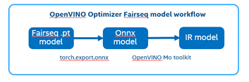
There are 2 steps to generate model ready for OpenVINO™ acceleration:
1. Use torch.export.onnx function convert the “.pt” model to “.onnx” model;
2. Use OpenVINO™ MO toolkit convert the “.onnx” model to “IR” model.
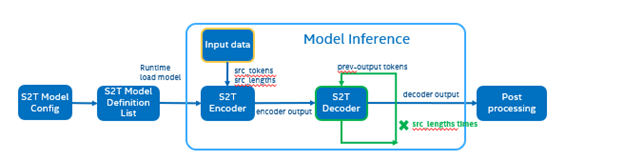
The following graph is the Fairseq framework inference workflow, it defines the model structure by “Model Config”, composes “Model Definition List” through multiple subgraph models, and dynamically loads the submodules in the model inference runtime.
Such as in the S2T task, model consists of two parts: Encoder and Decoder.
· Encoder is for extracting feature information from audio file.
· Decoder is for decoding the feature information to generate text information.
Fairseq Inference workflow
The length of audio information will affect the length of the feature information, and the length of the feature information will affect the Decoder submodule loop’s times. Therefore, the structure of the S2T model is dynamically defined according to the length of the input audio.
To optimize Fairseq framework model there’re 4 challenges need to be solved:
- Fairseq define submodules for various function, include variable in model layer define.
- Model structure is dynamically loaded in runtime and can’t export a whole torch model graph.
- Encoder and Decoder part models’ input shapes are dynamic, depending on input data size.
- Decoder part loop times depends by input sequence lengths.
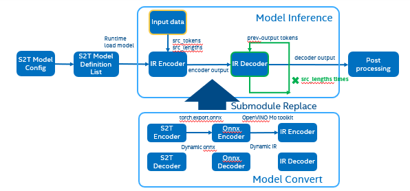
OpenVINO™ optimize Fairseq workflow
So that we should use some optimization tricks to solve these problems, to make sure the pipeline optimized by OpenVINO™.
- Divide model into Encoder and Decoder two parts, and separately export to onnx model,
- Because of the model structure define by input seq_len, should export dynamic shape onnx model.
- Convert onnx to IR model by OpenVINO™ MO toolkit.
- Replace the Fairseq S2T task pipeline Encoder and Decoder into IR model.
- Loading Inference Engine to run pipeline the pipeline on OpenVINO™.
Requirement
- Fairseq is a sequence modeling toolkit that allows researchers and developers to train custom models for translation, summarization, language modeling and other text generation tasks
- OpenVINO™ is an open-source toolkit for optimizing and deploying AI inference which can boost deep learning performance in computer vision, automatic speech recognition, natural language processing and other common task.
- Python version >=3.8
- PyTorch version >=1.10.0
Reference: GitHub: Fairseq-OpenVINO
Quick Start Demo
Step 1. Install fairseq and requirement
#Install OpenVINO™
Reference: Install OpenVINO by source code for Linux
Reference: Install OpenVINO by release package
Step 2. Download audio file and pre-train model file
In this blog we refer the “S2T Example: STon CoVoST” as sample, Preparation dataset and pre-train model can follow the Fairseq original step. Also, you can use “torch audio” to convert audio file to build customer dataset.
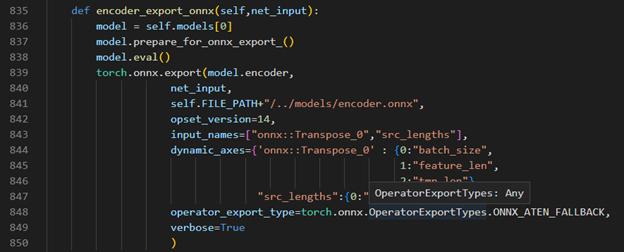
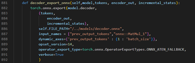
Step 3. Modify code to export onnx
Torch model export to onnx, We should adjust the contents in fairseq/sequence_generator.py +781 line "self.save_onnx = True" , +782 line "self.openvino_engine = False" The encoder.onnx and decoder.onnx will save in models
Encoder part model export to dynamic onnx
Decoder part model export to dynamic onnx
Step 4. Convert Model to IR
Convert encoder.onnx and decoder.onnx to encoder.xml and decoder.xml
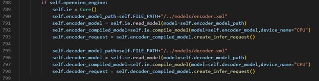
Step 5. OpenVINO™ Inference Engine optimize S2T pipeline
OpenVINO™ Inference S2T pipeline We should adjust the contents in fairseq/sequence_generator.py +781 line "self.save_onnx = False" , +782 line "self.openvino_engine =True" Use the converted the model to run OpenVINO™ Inference S2T pipeline.
OpenVINO™ Inference Engine initialization
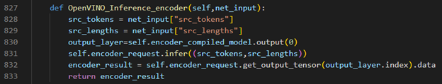
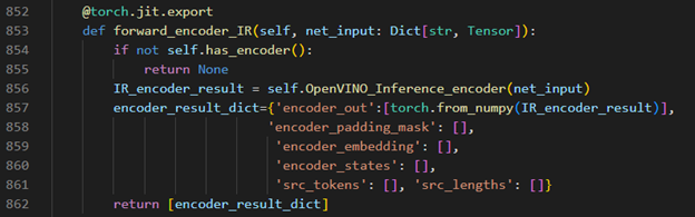
Encoder part inference by OpenVINO™
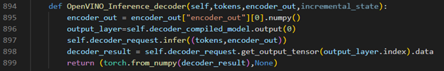
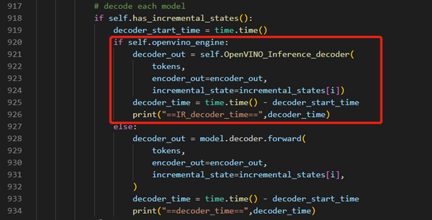
Decoder part inference by OpenVINO™
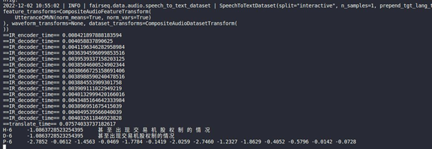
Inference Result
Extend OpenVINO™ to run PyTorch models with custom operations
Authors: Anna Likholat, Nico Galoppo
The OpenVINO™ Frontend Extension API lets you register new custom operations to support models with operations that OpenVINO™ does not support out-of-the-box. This article explains how to export the custom operation to ONNX, add support for it in OpenVINO™, and infer it with the OpenVINO™ Runtime.
The full implementation of the examples in this article can be found on GitHub in the openvino_contrib.
Export a PyTorch model to ONNX
Let's imagine that we have a PyTorch model which includes a new complex multiplication operation created by user (this operation was taken from DIRECT):
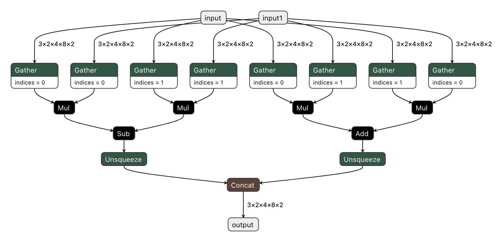
We'd like to export the model to ONNX and preserve complex multiplication operations as single fused nodes in the ONNX model graph, so that we can replace those nodes with custom OpenVINO operations down the line. If we were to export MyModel which directly calls the function above from its forward method, then onnx.export() would inline the PyTorch operations into the graph. This can be observed in the figure of the exported ONNX model below.
To prevent inlining of native PyTorch functions during ONNX export, we can wrap the function in a sub-class of torch.autograd.Function and define a static symbolic method. This method should return ONNX operators that represent the function's behavior in ONNX. For example:
You can find the full implementation of the wrapper class here: complex_mul.py
So now we're able to export the model with custom operation nodes to ONNX representation. You can reproduce this step with the export_model.py script:
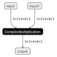
The resulting ONNX model graph now has a single ComplexMultiplication node, as illustrated below:
Enable custom operation for OpenVINO with Extensibility Mechanism
Now we can proceed with adding support for the ComplexMultiplication operation in OpenVINO. We will create an extension library with the custom operation for OpenVINO. As described in the Custom OpenVINO Operations docs, we start by deriving a custom operation class from the ov::op::Op base class, as in complex_mul.hpp.
1. Implement Operation Constructors
Implement the default constructor and constructors that optionally take the operation inputs and attributes as parameters. (code)
2. Override methods
2.1 validate_and_infer_types() method
Validates operation attributes and calculates output shapes using attributes of the operation: complex_mul.cpp.
2.2 clone_with_new_inputs() method
Creates a copy of the operation with new inputs: complex_mul.cpp.
2.3 has_evaluate() method
Defines the contstraints for evaluation of this operation: complex_mul.cpp.
2.4 evaluate() method
Implementation of the custom operation: complex_mul.cpp
3. Create an entry point
Create an entry point for the extension library with the OPENVINO_CREATE_EXTENSIONS() macro, the declaration of an extension class might look like the following:
This is implemented for the ComplexMultiplication operation in ov_extension.cpp.
4. Configure the build
Configure the build of your extension library using CMake. Here you can find the template of such script:
Also see an example of the finished CMake script for module with custom extensions here: CMakeLists.txt.
5. Build the extension library
Next we build the extension library using CMake. As a result, you'll get a dynamic library - on Linux it will be called libuser_ov_extensions.so, after the TARGET_NAME defined in the CMakeLists.txt above.
Deploy and run the custom model
You can deploy and run the exported ONNX model with custom operations directly with the OpenVINO Python API. Before we load the model, we load the extension library into the OpenVINO Runtime using the add_extension() method.
Now you're ready to load the ONNX model, and infer with it. You could load the model from the ONNX file directly using the read_model() method:
Alternatively, you can convert to an OpenVINO IR model first using Model Optimizer, while pointing at the extension library:
Note that in this case, you still need to load the extension library with the add_extension() method prior to loading the IR into your Python application.
The complete sequence of exporting, inferring, and testing the OpenVINO output against the PyTorch output can be found in the custom_ops test code.
See Also
Serving OpenVINO Models using the KServe API Standard
There are many network API specifications for model serving on the market today. Two of the most popular are TensorFlow Serving (TFS) and KServe. Starting with the 2022.2 release, OpenVINO Model Server supports KServe -- meaning both of these common API standards can be used for serving OpenVINO models. This blog explains how to take advantage of either API.
OpenVINO provides an efficient and high-performance runtime for executing deep learning inference. In many situations, AI applications need to delegate inference execution to a remote device or service over a network. There are many advantages to this approach including the ability to scale.
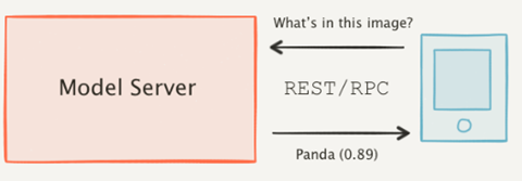
AI software developers expect the communication interface with a model server to remain stable. In many cases, developers want to perform pre/post-processing on the client side with minimal dependencies. They are reluctant to switch to a different serving implementation if that requires substantial code changes or new dependencies in their applications.
Since the first release in 2018, OpenVINO Model Server has supported the TFS API. And as of 2022, the KServe API is now supported as well.
KServe is a standard designed by several companies across the industry. It has been adopted by model servers like Triton Inference Server and TorchServe. Now the same client can easily switch to use OpenVINO Model Server and leverage the latest optimizations in Intel(R) CPUs and GPUs.
KServe Python Example
Below is a simple example how to use KServe using the Python-based tritonclient.
Create Model Repository
Start OpenVINO Model Server with a ResNet-50 Model:
Install Python Client Library
Get the Model Metadata
Get a Sample Image

Run Inference via gRPC Interface with a NumPy File as Input Data
Run Inference via REST Interface with a JPEG File as Input Data
Run Inference via REST Interface with a JPEG File as Input Data using cURL
KServe C++ Example
The inference execution is also made easy in C++ based client applications. The examples below show client application execution based on the Triton C++ client library.
Build the Samples:
Get the Model Metadata
The compiled application grpc_model_metadata can make a call to gRPC endpoint and query for a server model metadata.
Run Inference via gRPC with a JPEG Encoded File as the Input Data
The sample application grpc_infer_resnet is sending the inference requests for a set of images listed inresnet_input_images.txt including their expected classification number in the ImageNet dataset.
In addition to the KServe API, the TFS API can still be used by client applications. This gives you the option to use a range of client libraries like tensorflow-serving-api or the much lighter and simplified ovmsclient.
To help you get started, we provide samples in Python, C++, Java and Go:
In conclusion, it is now easier to connect and AI applications to OpenVINO Model Server. In existing applications, you can even use the same code to take advantage of the benefits of OpenVINO.
Use Metrics to Scale Model Serving Deployments in Kubernetes
In this blog you will learn how to set up horizontal autoscaling in Kubernetes using inference performance metrics exposed by OpenVINO™ Model Server. This will enable efficient scaling of model serving pods for inference on Intel® CPUs and GPUs.
Why use custom metrics?
OpenVINO™ Model Server provides high performance AI inference on Intel CPUs and GPUs that can be scaled in Kubernetes. However, when it comes to automatic scaling in Kubernetes, the Horizontal Pod Autoscaler by default, relies on CPU utilization and memory usage metrics only. Although resource consumption indicates how busy the application is, it does not clearly say whether serving provides expected quality of service to the clients or not. Since OpenVINO Model Server exposes performance metrics, we can automatically scale based on service quality rather than resource utilization.
The first metric that comes to mind when thinking about service performance is the duration of request processing, otherwise known as latency. For example, mean or median over a specified period or latency percentiles. OpenVINO Model Server provides such metrics but setting autoscaling based on latency requires specific knowledge about each model and the environment where the inference is running in order to properly set thresholds that trigger scaling.
While autoscaling based on latency works and may be a good choice when you have model-specific knowledge, we will instead focus on a more generic metric using ovms_requests_streams_ratio. Let’s dive into what this means.
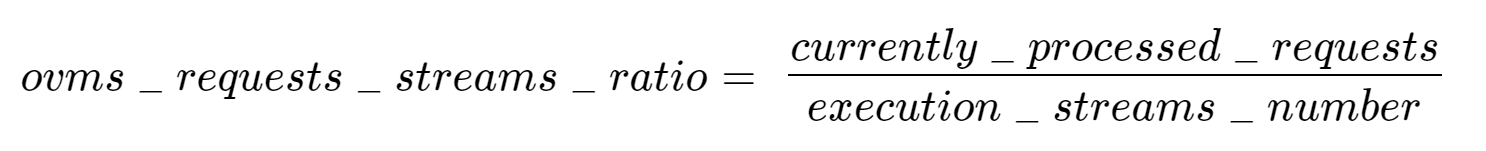
In the equation above:
- currently_processed_requests - number of inference requests to a model being processed by the service at a given time.
- execution_streams_number – number of execution streams. (When a model is loaded on the device, its computing units are divided into streams. Each stream independently handles inference requests, meaning that the number of streams defines how many inferences can be run on the device in parallel. Note that the more streams there are, the less powerful they are, so we get more throughput at a cost of higher minimal latency / inference time.)
In this equation, for any model exceeding a value of 1 indicates that requests are starting to queue up. Setting the autoscaler threshold for the ovms_requests_streams_ratio metric is somewhat of an arbitrary decision that should be made by a cluster administrator. Setting the threshold too low will result in underutilization of nodes and setting it too high will force the system to work with insufficient resources for extended periods of time. Now that we have chosen a metric for autoscaling, let’s start setting it up.
Deploy Model Server with Autoscaling Metrics
First, we need to create a deployment of OpenVINO Model Server in Kubernetes. To do this, follow instructions to install the OpenVINO Operator in your Kubernetes cluster. Then create a configuration where we can specify the model to be served and enable metrics:
Create ConfigMap:
With the configuration in place, we can deploy OpenVINO Model Server instance:
Create ModelServer resource:
Deploy and Configure Prometheus
Next, we need to read serving metrics and expose them to the Horizontal Pod Autoscaler. To do this we will deploy Prometheus to collect serving metrics and the Prometheus Adapter to expose them to the autoscaler.
Deploy Prometheus Monitoring Tool
Let’s start with Prometheus. In the example below we deploy a simple Prometheus instance via the Prometheus Operator. To deploy the Prometheus Operator, run the following command:
Next, we need to configure role-based access control to give Prometheus permission to access the Kubernetes API:
The last step is to create a Prometheus instance by deploying Prometheus resource:
If the deployment was successful, a Prometheus service should be running on port 9090. You can set up a port forward for this service, enabling access to the web interface via localhost on your machine:
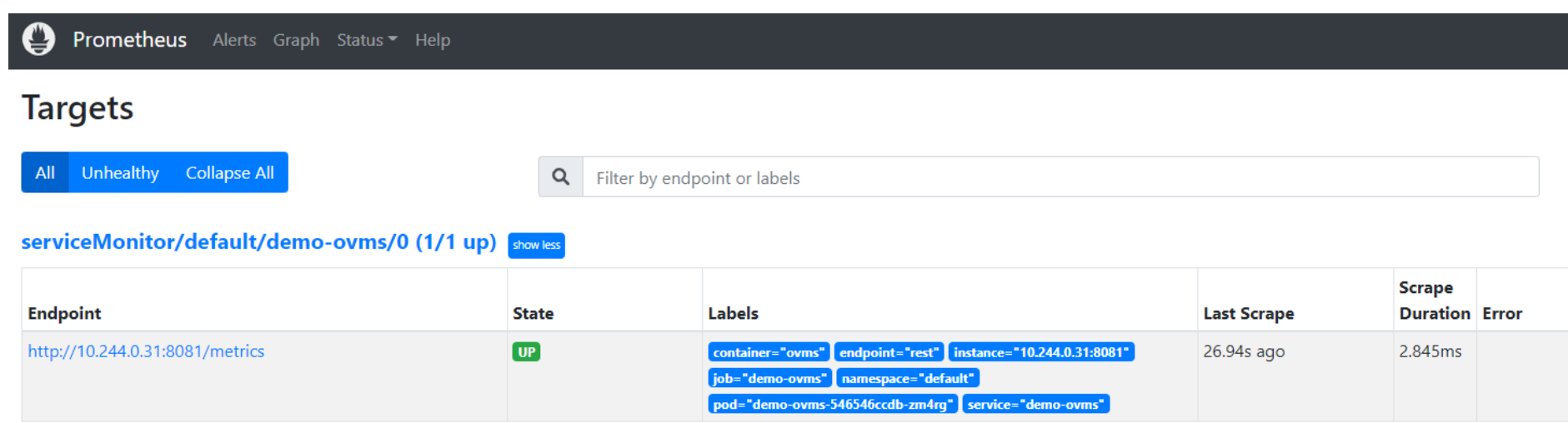
Now, when you open http://localhost:9090 in a browser you should see the Prometheus user interface. Next, we need to expose the Model Server to Prometheus by creating a ServiceMonitor resource:
Once it’s ready, you should see a demo-ovms target in the Prometheus UI:
Now that the metrics are available via Prometheus, we need to expose them to the Horizonal Pod Autoscaler. To do this, we deploy the Prometheus Adapter.
Deploy Prometheus Adapter
Prometheus Adapter can be quickly installed via helm or step-by-step via kubectl. For the sake of simplicity, we will use helm3. Before deploying the adapter, we will prepare a configuration that tells it how to expose the ovms_requests_streams_ratio metric:
Create a ConfigMap:
Now that we have a configuration, we can install the adapter:
Keep checking until custom metrics are available from the API:
Once you see the output above, you can configure the Horizontal Pod Autoscaler to use these metrics.
Set up Horizontal Pod Autoscaler
As mentioned previously, we will set up autoscaling based on the ovms_requests_streams_ratio metric and target an average value of 1. This will try to keep all streams busy all the time while preventing requests from queueing up. We will set minimum and maximum number of replicas to 1 and 3, respectively, and the stabilization window for both upscaling and downscaling to 120 seconds:
Create HorizontalPodAutoscaler:
Once deployed, you can generate some load for your model and see the results. Below you can see how Horizontal Pod Autoscaler scales the number of replicas by checking its status:

This data can also be visualized with a Grafana dashboard:
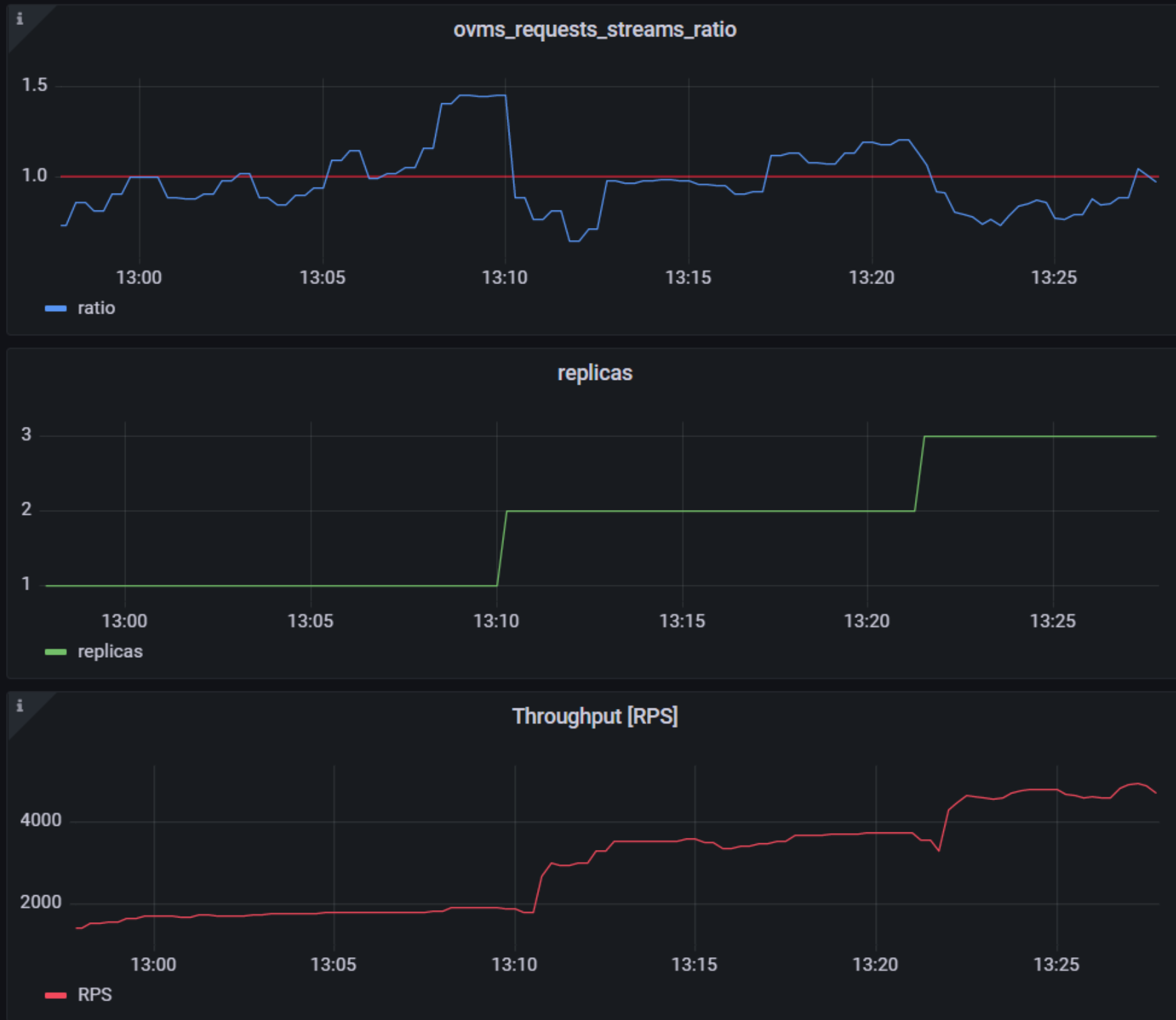
As you can see, with OpenVINO Model Server metrics, you can quickly set up inferencing system with monitoring and autoscaling for any model. Moreover, with custom metrics, you can set up autoscaling for inference on any Intel CPUs and GPUs.
See also:
- Load Balancing OpenVINO Model Server Deployments with Red Hat
- Kubernetes Device Plugin for Intel GPU
- OpenVINO Model Server metrics