

OpenVINO Blog
OpenVINO optimizer Latent Diffusion Models (LDM) for super-resolution
OpenVINO optimizer Latent Diffusion Models(LDM) for super-resolution
Introduction
A computer vision approach called image super-resolution aims to increase the resolution of low-resolution images so that they are clearer and more detailed. Applicationsfor super-resolution include the processing of medical images, surveillancefootage, and satellite images.
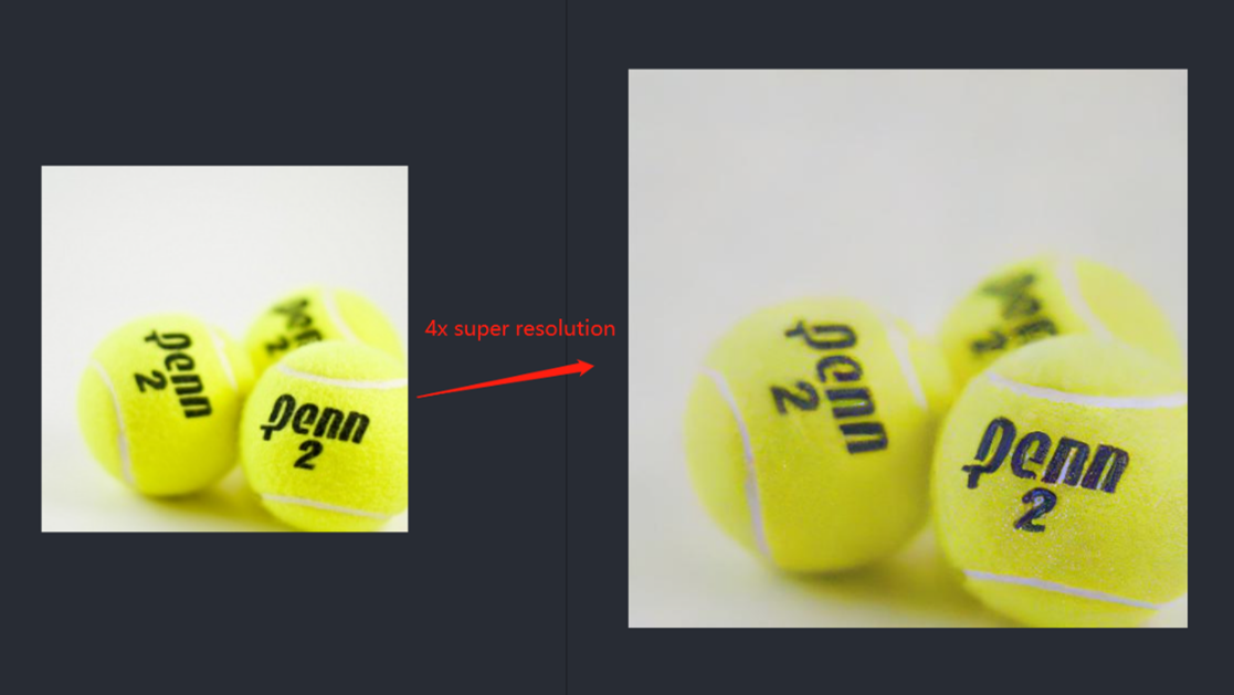
The LDM (LatentDiffusion Models) Super Resolution model, a deep learning-based approach to photo super-resolution, was developed by the Hugging Face Research team. The residual network (ResNet) architecture, a type of convolutional neural network(CNN) created to address the issue of vanishing gradients in deep neuralnetworks.
Diffusion models are generative models,meaning that they are used to generate data similar to the data on which they are trained. Fundamentally, Diffusion Models work by destroying training data through the successive addition of Gaussian noise, andthen learning to recover the data by reversing this noising process. After training, we can use the Diffusion Model to generatedata by simply passing randomly sampled noise through the learned denoising process.

Diffusion Model is a latent variable model which maps to the latent space using a fixed Markov chain. This chain gradually adds noise to thedata in order to obtain the approximate posterior.

Ultimately, the image is asymptotically transformed to pure Gaussian noise. The goal of training a diffusion model is to learn the reverse process. By traversing backward along this chain, we can generate new data.

Requirement
- Optimum-intel Optimum Intel is the interface betweenthe HuggingFace Transformers and Diffusers libraries and the differenttools and libraries provided by Intel to accelerate end-to-end pipelines onIntel architectures.
Intel Neural Compressor is an open-source library enabling the usageof the most popular compression techniques such as quantization, pruning and knowledge distillation
- OpenVINO™ is an open-sourcetoolkit for optimizing and deploying AI inference which can boost deep learningperformance in computer vision, automatic speech recognition, natural language processing and other common task.
- optimum-intel==1.5.2(include openvino)
- openvino
- openvino-dev
- diffusers
- pytorch >= 1.9.1
- onnx >= 1.13.0
Reference: optimum-intel-ldm-super-resolution-4x
QuickStart Demo
Original repo is from HuggingFace CompVis/ldm-super-resolution-4x-openimages,we are reference to build our pipeline to implement super-resolution related function.
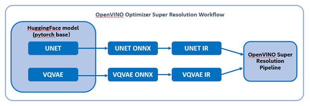
To transformand acceleration optimize the pipeline by openvino, there are 3 steps need to do.
- Step1. Install the requirement package and initial environment.
- Step2. Convert original model to openvino IR model.
- Step3. Build OpenVINO super resolution pipeline.
Now, Let’s start with the content of our tutorial.
Step 1. Install the requirementpackage and initial environment
OpenVINO has the standard installation process, we can directly refer tothe official OpenVINO documentation to install.
Reference: Install OpenVINO by source code for Linux
Reference: Install OpenVINO by release package
Optimum Intel also can refer the standard guide.
Reference: Optimum-intel install guide
(Optional) Install the latest stable release by pipe :
# pip install openvino, openvino-dev
# pip install"optimum[openvino,nncf]"
Step 2. Convert originalmodel to OpenVINO IR model
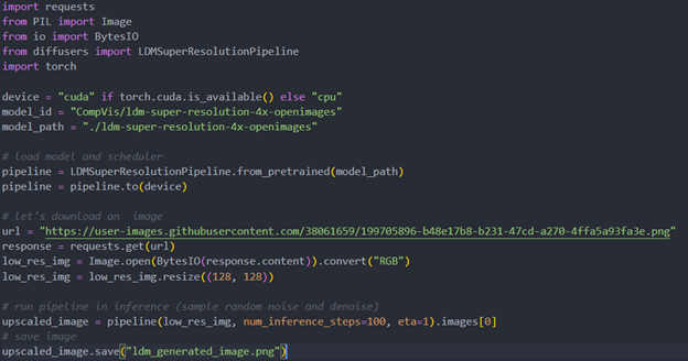
Firstly, run pipe the HuggingFace pipeline, it will automate download the models, and we need to convert them from pytorch->onnx->IR, to enable the model by OpenVINO.
%20workflow.png)
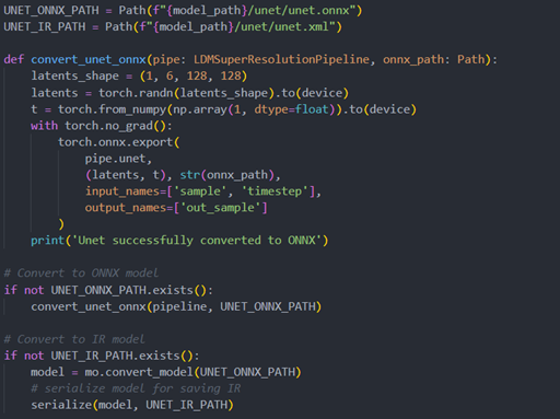
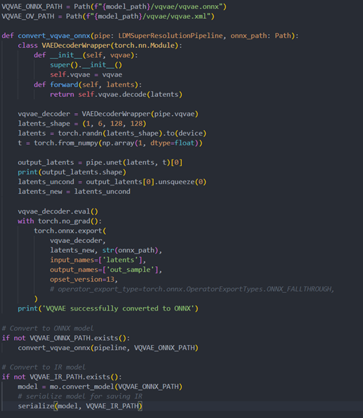
The LDM (LatentDiffusion Models) Super Resolution model has two part of sub-models: unet and vqvae,we should convert each of them in to IR model.
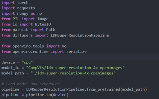
The reference source code for model convert,also we provide the script in the GitHub repo : ov-ldm4x-model-convert.py
Initial parameter and the ov-pipeline
Unet sub-model convert to IR
Vqvae sub-model convert to IR
Step 3. Build OpenVINOsuper resolution pipeline
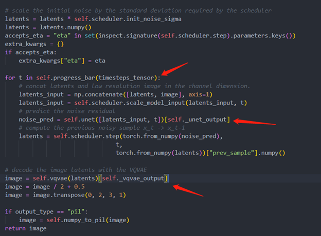
The LDM (Latent Diffusion Models) Super Resolution OpenVINO pipeline main function part code, the whole pipeline script is provided in GitHub repo: ov-ldm4x-pipeline.py
Inference Result

Deploy End to End Super-Resolution Pipeline with OpenVINO™ Model Server
Introduction
In this blog, we will show how to deploy an end-to-end super-resolution pipeline by leveraging OpenVINOTM Model Server with Demultiplexing in DAG and Custom Node features.
OpenVINOTM Model Server (OVMS) is a high-performance system for serving models that uses the same architecture and API as TensorFlow Serving and KServe while applying OpenVINOTM for inference execution. It is implemented in C++ for scalability and optimized for deployment on intel architectures.
Directed Acyclic Graph (DAG) is an OVMS feature that controls the execution of an entire graph of interconnected models defined within the OVMS configuration. The DAG scheduler makes it possible to create a pipeline of models for execution in the server with a single client request.
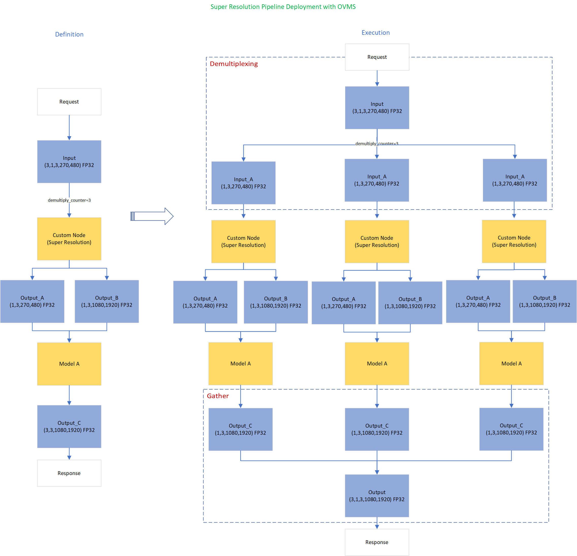
During the pipeline execution, it is possible to split a request with multiple batches into a set of branches with a single batch. Internally, OVMS demultiplexer will divide the data, process them in parallel and combine the results.
The custom node in OVMS simplifies linking deep learning models into complete pipeline. Custom node can be used to implement all operations on the data which cannot be handled by the neural network model. It is represented by a C++ dynamic library implementing OVMS API defined in custom_node_interface.h.
Super-Resolution Pipeline Workflow
Figure1 shows the super-resolution pipeline in a flowchart, where we use "demultiply_counter=3" without loss of generality. The whole pipeline starts with input data from the Request node via gRPC calls. Batched input data with 5D shape(3,1,3,270,480) is split into a single batch by the DAG demultiplexer. Each single batch of data is fed into a custom node for image preprocessing. The two outputs of the custom node serve as inputs for model A inference. In the end, all inference results are gathered as output C, which will be sent by the Response node to the client via gRPC calls.
Here is an example configuration for the super-resolution pipeline deployed with OVMS.
“pipeline_config_list” contains super-resolution pipeline information, data enter from the “request” node, flow to “sr_preprocess_node” for image preprocessing, generated two outputs will serve as inputs in “super_resolution_node” for inference, gathered inference results will be returned by “response” node.
- "demultiply_count": acceptable input data batch size when Demultiplexing in DAG feature enabled, “demultiply_count” with value -1 means OVMS can accept dynamic batch input data.
“model_config_list”: contains the basic configuration for super-resolution deep learning model and OpenVINOTM CPU plugin configuration.
- "nireq": set number of infer requests used in OVMS server for deep learning model
- "NUM_STREAMS": set number of streams used in the CPU plugin
- "INFERENCE_PRECISION_HINT": option to select preferred inference precision in CPU plugin. We can set "INFERENCE_PRECISION_HINT":bf16 on the Xeon platform that supports BF16 precision, such as the 4th Gen Intel® Xeon® Scalable processor (formerly codenamed Sapphire Rapids). Otherwise, we should set "INFERENCE_PRECISION_HINT":f32 as the default value.
“custom_node_library_config_list”: contains the name and path of the custom node dynamic library
Image Preprocessing with libvips in Custom Node
In this blog, we use a single-image-super-resolution model from Open Model Zoo for the super-resolution pipeline. The model requires two inputs according to the model specification. The first input is the original image (shape [1,3,270,480]). The second input is a 4x resized image with bicubic interpolation (shape [1,3,1080,1920]). Both input images expected color space is BGR. Therefore, image preprocessing for input image is required.
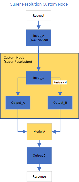
Figure2 shows the custom node designed for image preprocessing in the super-resolution pipeline. The custom node takes the original input image as input data. At first, input data is assigned to output 1 without modification. Besides, the input data is resized 4x with bicubic interpolation and assigned as output 2. The two outputs are passed to the model node for inference. For image processing in the custom node, we utilize libvips – an open-source image processing library that is designed to be fast and efficient with low memory usage. Please see the detailed custom node implementation in super_resolution_nhwc.cpp.
Although libvips is very sufficient for image processing operations with less memory, libvips does not provide functionality for layout (NCHW->NHWC) and color space (RGB->BGR) conversion, which is required by the super-resolution model as inputs. Instead, we can integrate layout and color space conversion into models using OpenVINOTM Preprocessing API.
Integrate Preprocessing with OpenVINOTM Preprocessing API
OpenVINOTM Preprocessing API allows adding custom preprocessing steps into the execution graph of OpenVINOTM models.
Here is a sample code to integrate layout (NCHW-> NHWC) and color space (BRG->RGB) conversion into the super-resolution model with OpenVINOTM Preprocessing API.
In the code snippet above, we first load the original model and initialize the PrePostProcessor object with the original model. Then we modify the model's 1st input element type to “uint8”, change the color format from the default “BGR” to “RGB”, and set the layout from “NCHW” to “NHWC”. In the end, we build a new model and serialize it on the disk. The whole model preprocessing can be done offline, please find details in model_preprocess.py.
Build Model Server Docker Image for Super-Resolution Pipeline
Build OVMS docker image with custom node
Copy compiled custom nodes library to the “models” directory
Setup client environment
Integrate preprocessing with OpenVINOTM Preprocessing API
The resulting model will be saved in the “super_resolution_model_preprocessed/1” directory.
Super-Resolution Pipeline Demo
Start the OpenVINOTM Model Server with docker binding with 8 cores
Run client with command line
Figure 3 shows the original input image (shape 270x480).

Figure 4 shows the resized image (shape 1080x1920) after image preprocessing in the custom node.

Figure 5 shows the inference result of the super-resolution model (shape1080x1920).

Conclusion
In this blog, we demonstrate an end-to-end super-resolution pipeline deployment with OpenVINOTM Model Server. The whole pipeline takes dynamic batched images (RGB, NHWC) as input, demultiplexing into single batch data, preprocess with a custom node, runs an inference with a super-resolution model, send gathered inference results to the client in the end.
This blog provides following examples that utilize OpenVINOTM Model Server and OpenVINOTM features:
- Enable OVMS DAG demultiplexing feature
- Provide custom node for image preprocessing using libvips
- Provide sample code for integrating preprocessing into the model with OpenVINOTM Preprocessing API.
- Support super-resolution end-to-end pipeline with image preprocessing and model inference with OVMS DAG scheduler
Remote Tensor API Sample
This AI pipeline implements zero-copy between SYCL and OpenVINO through the Remote Tensor API of the GPU Plugin.
- Introduction
The development of SYCL simplifies the use of OpenCL, which can fully exploit the computing power of GPU in the pipeline. Meanwhile, SYCL has more flexibility to do customized pre- and post-processing of OpenVINO. To further optimize the pipeline, developers can use GPU Plugin to avoid the memory copy overhead between SYCL and OpenVINO. The GPU plugin provides the ov::RemoteContext and ov::RemoteTensor interfaces for video memory sharing and interoperability with existing native APIs, such as OpenCL, Microsoft DirectX, or VAAPI. For details, please refer to the online documentation of OpenVINO.
Based on the pseudocode of the online documentation, here we provide a simple pipeline sample with Remote Tensor API. Because in the rapid iteration of oneAPI, sometimes customers need quick verification so that this sample can be used for testing. OneAPI also provides a real-world, end-to-end example, which optimizes PointPillars for lidar object detection.
- Components
SYCL preprocessing is based on the Sepia Filter sample, which demonstrates how to convert a color image to a Sepia tone image, a monochromatic image with a distinctive Brown Gray color. The sample program works by offloading the compute-intensive conversion of each pixel to Sepia tone using SYCL*-compliant code for CPU and GPU.
OpenVINO inferencing is based on the OpenVINO classification sample, the input from SYCL filtered image in the device will be sent into OpenVINO as a remote tensor without a memory copy.
Remote Tensor API: Create RemoteContext from SYCL pre-processing’s native handle. After model compiling, do memory sharing between the application and GPU plugin with from cl::Buffer to remote tensor.
- Build Sample on Linux
Download the source code from the link. Prepare the model and images.
To run the sample, you need to specify a model and image:
Use pre-trained models from the Open Model Zoo. The models can be downloaded using the Model Downloader. Use images from the media files collection.
Run on Intel NUC Core 11 iGPU with OpenVINO 2022.2 and oneAPI 2022.3.
./intel64/hello_nv12_input_classification_oneAPI../model/FP32/alexnet.xml ../image/dog512.bmp GPU 2
Sample Output:
Warning: With the updating of OpenVINO and oneAPI, different versions may cause problems with the tools in the common directory or the new SYCL header name. Please use the same version or debug following the corresponding release instructions.
Accelerate Inference of Sparse Transformer Models with OpenVINO™ and 4th Gen Intel® Xeon® Scalable Processors
Authors: Alexander Kozlov, Vui Seng Chua, Yujie Pan, Rajesh Poornachandran, Sreekanth Yalachigere, Dmitry Gorokhov, Nilesh Jain, Ravi Iyer, Yury Gorbachev
Introduction
When it comes to the inference of overparametrized Deep Neural Networks, perhaps, weight pruning is one of the most popular and promising techniques that is used to reduce model footprint, decrease the memory throughput required for inference, and finally improve performance. Since Language Models (LMs) are highly overparametrized and contain lots of MatMul operations with weights it looks natural to prune the redundant weights and benefit from sparsity at inference time. There are several types of pruning methods available:
- Fine-grained pruning (single weights).
- Coarse pruning: group-level pruning (groups of weights), vector pruning (rows in weights matrices), and filter pruning (filters in ConvNets).
Contemporary Language Models are basically represented by Transformer-based architectures. Using coarse pruning methods for such models is problematic because of the many connections between the layers. This trait means that, first, not every pruning type is applicable to such models and, second, pruning of some dimension in one layer requires adjustments in the rest of the layers connected to it.
Fine-grained sparsity does not have such a constraint and can be applied to each layer independently. However, it requires special support on the HW and inference SW level to get real performance improvements from weight sparsity. There are two main approaches that help to leverage from weight sparsity at inference:
- Skip multiplication and addition for zero weights in dot products of weights and activations. This usually results in a special instruction set that implements such logic.
- Weights compression/decompression to reduce the memory throughput. Compression is performed at the model load/compilation stage while decompression happens on the fly right before the computation when weights are in the cache. Such a method can be implemented on the HW or SW level.
In this blog post, we focus on the SW weight decompression method and showcase the end-to-end workflow from model optimization to deployment with OpenVINO.
Sparsity support in OpenVINO
Starting from OpenVINO 2022.3release, OpenVINO runtime contains a feature that enables weights compression/decompression that can lead to performance improvement on the 4thGen Intel® Xeon® Scalable Processors. However, there are some prerequisites that should be considered to enable this feature during the model deployment:
- Currently, this feature is available only to MatMul operations with weights (Fully-connected layers). So currently, there is no support for sparse Convolutional layers or other operations.
- MatMul layers should contain a high level of weights sparsity, for example, 80% or higher which is achievable, especially for large Transformer models trained on simple tasks such as Text Classification.
- The deployment scenario should be memory-bound. For example, this prerequisite is applicable to cloud deployment when there are multiple containers running inference of the same model in parallel and competing for the same RAM and CPU resources.
The first two prerequisites assume that the model is pruned using special optimization methods designed to introduce sparsity in weight matrices. It is worth noting that pruning methods require model fine-tuning on the target dataset in order to reduce accuracy degradation caused by zeroing out weights within the model. It assumes the availability of the HW capable of DL model training. Nowadays, many frameworks and libraries offer such methods. For example, PyTorch provides some capabilities for NN pruning. There are also resources that offer pre-trained sparse models that can be used as a starting point, for example, SparseZoo from Neural Magic.
OpenVINO also provides instruments for DL model pruning implemented in Neural Network Compression Framework (NNCF) that is aimed specifically for model optimization and offers different optimization options: from post-training optimization to deep compression when stacking several optimization methods. NNCF is also integrated into Hugging Face Optimum library which is designed to optimize NLP models from Hugging Face Hub.
Using only sparsity is not so beneficial compared to another popular optimization method such as bit quantization which can guarantee better performance-accuracy trade-offs after optimization in the general case. However, the good thing about sparsity is that it can be stacked with 8-bit quantization so that the performance improvements of one method reinforce the optimization effect of another one leading to a higher cumulative speedup when applying both. Considering this, OpenVINO runtime provides an acceleration feature for sparse and 8-bit quantized models. The runtime flow is shown in the scheme below:
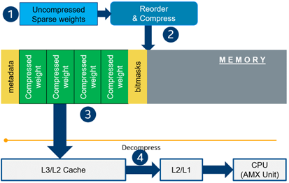
Below, we demonstrate two end-to-end workflows:
- Pruning and 8-bit quantization of the floating-point BERT model using Hugging Face Optimum and NNCF as an optimization backend.
- Quantization of sparse BERT model pruned with 3rd party optimization solution.
Both workflows end up with inference using OpenVINO API where we show how to turn on a runtime option that allows leveraging from sparse weights.
Pruning and 8-bit quantization with Hugging Face Optimum and NNCF
This flow assumes that there is a Transformer model coming from the Hugging Face Transformers library that is fine-tuned for a downstream task. In this example, we will consider the text classification problem, in particular the SST2 dataset from the GLUE benchmark, and the BERT-base model fine-tuned for it. To do the optimization, we used an Optimum-Intel library which contains the optimization capabilities based on the NNCF framework and is designed for inference with OpenVINO. You can find the exact characteristics and steps to reproduce the result in this model card on the Hugging Face Hub. The model is 80% sparse and 8-bit quantized.
To run a pre-optimized model you can use the following code from this notebook:
Quantization of already pruned model
In case if you deal with already pruned model, you can use Post-Training Quantization from the Optimum-Intel library to make it 8-bit quantized as well. The code snippet below shows how to quantize the sparse BERT model optimized for MNLI dataset using Neural Magic SW solution. This model is publicly available so that we download it using Optimum API and quantize on fly using calibration data from MNLI dataset. The code snippet below shows how to do that.
Enabling sparsity optimization inOpenVINO Runtime and 4th Gen Intel® Xeon® Scalable Processors
Once you get ready with the sparse quantized model you can use the latest advances of the OpenVINO runtime to speed up such models. The model compression feature is enabled in the runtime at the model compilation step using a special option called: “CPU_SPARSE_WEIGHTS_DECOMPRESSION_RATE”. Its value controls the minimum sparsity rate that MatMul operation should have to be optimized at inference time. This property is passed to the compile_model API as it is shown below:
An important note is that a high sparsity rate is required to see the performance benefit from this feature. And we note again that this feature is available only on the 4th Gen Intel® Xeon® Scalable Processors and it is basically for throughput-oriented scenarios. To simulate such a scenario, you can use the benchmark_app application supplied with OpenVINO distribution and limit the number of resources available for inference. Below we show the performance difference between the two runs sparsity optimization in the runtime:
- Benchmarking without sparsity optimization:
- Benchmarking when sparsity optimization is enabled:
Performance Results
We performed a benchmarking of our sparse and 8-bit quantized BERT model on 4th Gen Intel® Xeon® Scalable Processors with various settings. We ran two series of experiments where we vary the number of parallel threads and streams available for the asynchronous inference in the first experiments and we investigate how the sequence length impact the relative speedup in the second series of experiments.
The table below shows relative speedup for various combinations of number of streams and threads and at the fixed sequence length after enabling sparsity acceleration in the OpenVINO runtime.
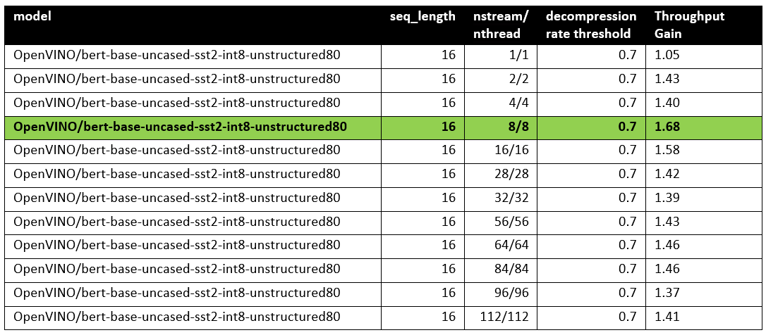
Based on this, we can conclude that one can expect significant performance improvement with any number of streams/threads larger than one. The optimal performance is achieved at eight streams/threads. However, we would like to note that this is model specific and depends on the model architecture and sparsity distribution.
The chart below also shows the relationship between the possible acceleration and the sequence length.
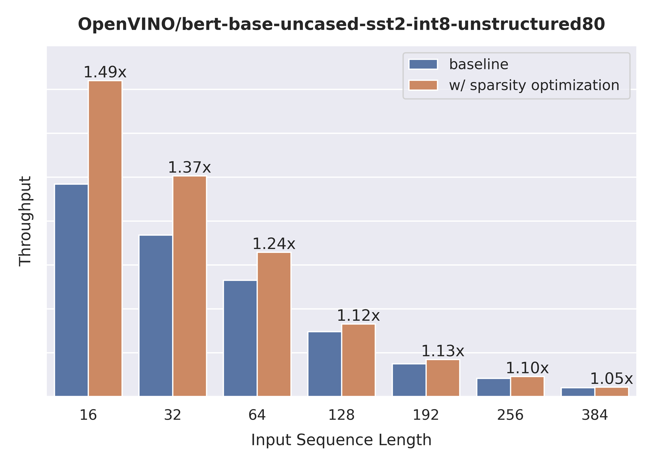
As you can see the benefit from sparsity is decreasing with the growth of the sequence length processed by the model. This effect can be explained by the fact that for larger sequence lengths the size of the weights is no longer a performance bottleneck and weight compression does not have so much impact on the inference time. It means that such a weight sparsity acceleration feature does not suit well for large text processing tasks but could be very helpful for Question Answering, Sequence Classification, and similar tasks.
References
OpenVINO™ Enable PaddlePaddle Quantized Model
OpenVINO™ is a toolkit that enables developers to deploy pre-trained deep learning models through a C++ or Python inference engine API. The latest OpenVINO™ has enabled the PaddlePaddle quantized model, which helps accelerate their deployment.
From floating-point model to quantized model in PaddlePaddle
Baidu releases a toolkit for PaddlePaddle model compression, named PaddleSlim. The quantization is a technique in PaddleSlim, which reduces redundancy by reducing full precision data to a fixed number so as to reduce model calculation complexity and improve model inference performance. To achieve quantization, PaddleSlim takes the following steps.
- Insert the quantize_linear and dequantize_linear nodes into the floating-point model.
- Calculate the scale and zero_point in each layer during the calibration process.
- Convert and export the floating-point model to quantized model according to the quantization parameters.
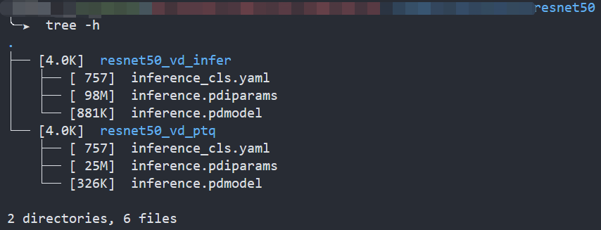
As the Figure1 shows, Compared to the floating-point model, the size of the quantized model is reduced by about 75%.
Enable PaddlePaddle quantized model in OpenVINO™
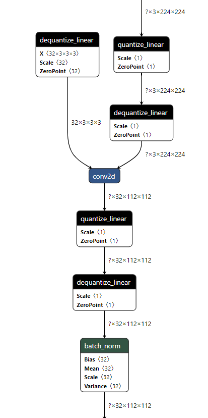
As the Figure2.1 shows, paired quantize_linear and dequantize_linear nodes appear intermittently in the model.
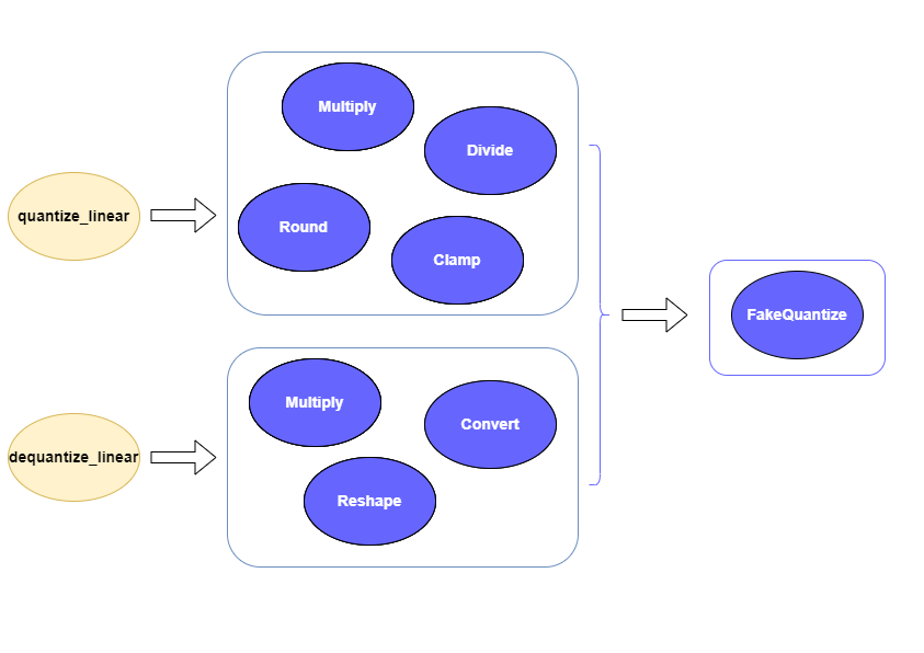
In order to enable PaddlePaddle quantized model, both quantize_linear and dequantize_linear nodes should be mapped first. And then, quantize_linear and dequantize_linear pattern scan be fused into FakeQuantize nodes and OpenVINO™ transformation mechanism will simplify and optimize the model graph in the quantization mode.
To check the kernel execution function, just profile and dump the execution progress, you can use benchmark_app as an example. The benchmark_app provides the option"-pc", which is used to report the performance counters information.
- To report the performance counters information of PaddlePaddle resnet50 float model, we can run the command line:

- To report the performance counters information of PaddlePaddle resnet50 quantized model, we can run the command line:

By comparing the Figure2.3 and Figure2.4, we can easily find that the hotpot layers of PaddlePaddle quantized model are dispatched to integer ISA implementation, which can accelerate the execution.
Accuracy
We compare the accuracy between resnet50 floating-point model and post training quantization(PaddleSlim PTQ) model. The accuracy of PaddlePaddle quantized model only decreases slightly, which is expected.
Performance
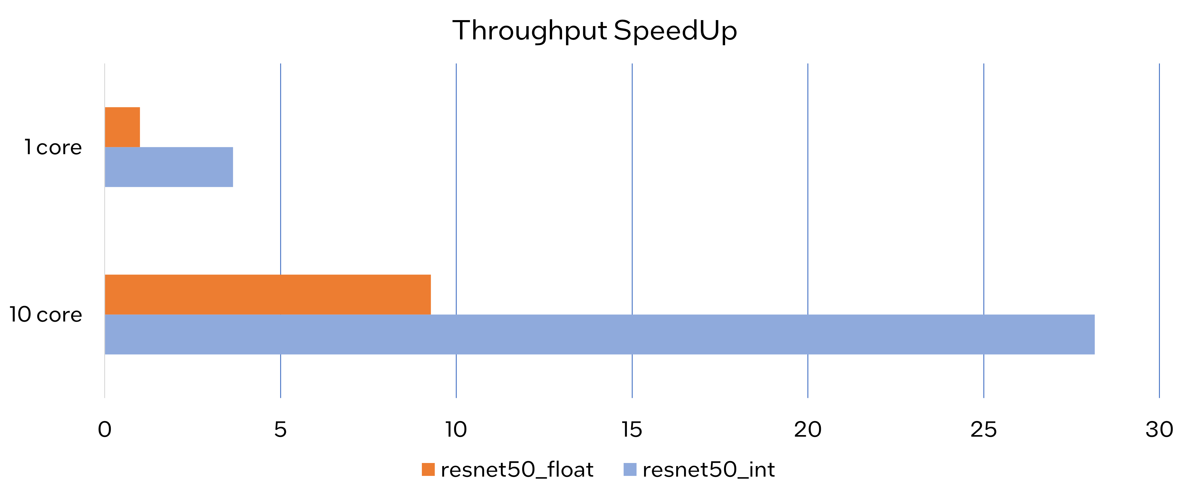
Throughput Speedup
The throughput of PaddlePaddle quantized resnet50 model can improve >3x.
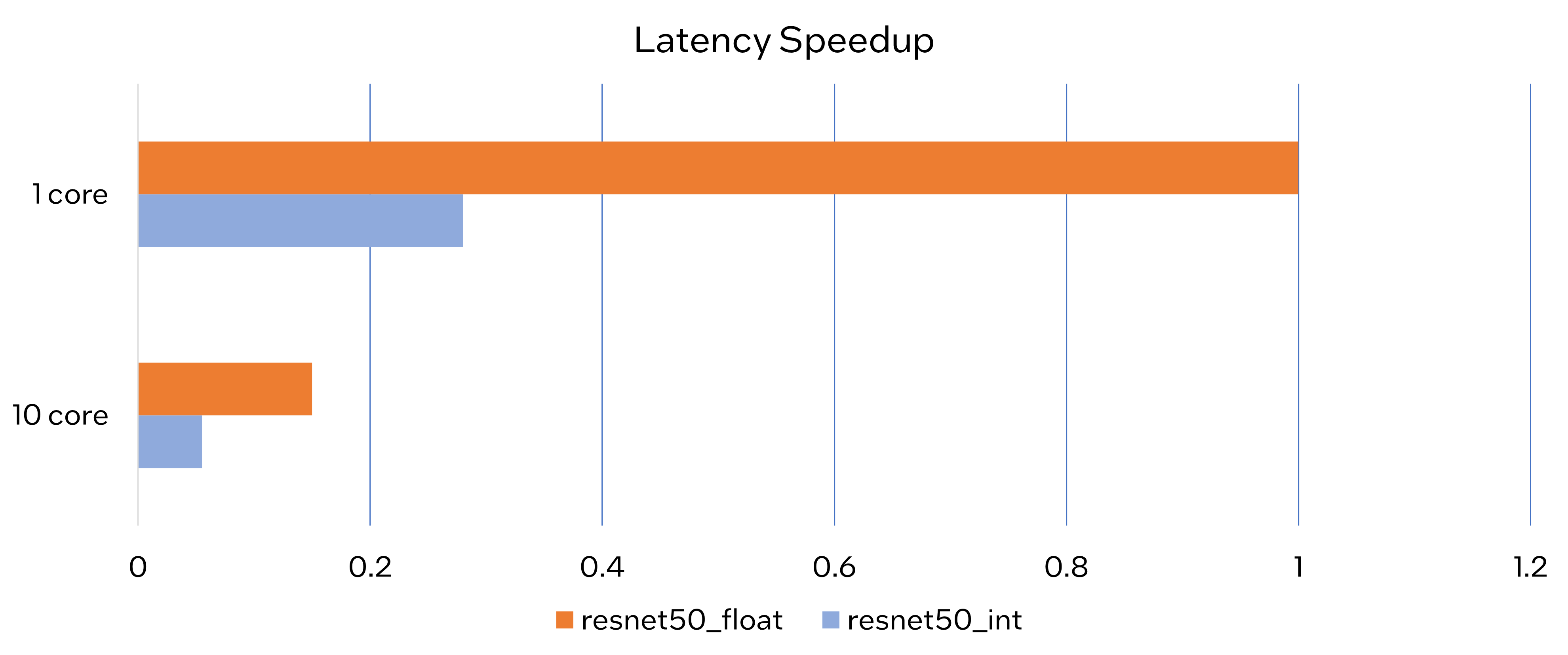
Latency Speedup
The latency of PaddlePaddle quantized resnet50 model can reduce about 70%.
Conclusion
In this article, we elaborated the PaddlePaddle quantized model in OpenVINO™ and profiled the accuracy and performance. By enabling the PaddlePaddle quantized model in OpenVINO™, customers can accelerate both throughput and latency of deployment easily.
Notices & Disclaimers
- The accuracy data is collected based on 50000 images of val dataset in ILSVRC2012.
- The throughput performance data is collected by benchmark_app with data_shape "[1,3,224,224]" and hint throughput.
- The latency performance data is collected by benchmark_app with data_shape "[1,3,224,224]" and hint latency.
- The machine is Intel® Xeon® Gold 6346 CPU @3.10GHz.
- PaddlePaddle quantized model can be achieve at https://github.com/PaddlePaddle/FastDeploy/blob/develop/docs/en/quantize.md.
Benchmark_app Servers Usage Tips with Low-level Setting for CPU
We provide tips for Benchmark_app in different situations like VPS and bare metal servers. The tips aim at practical evaluation with limited hardware resources. Help customers quickly balance performance and hardware resource requirements when deploying AI on servers. Besides the suggestion of different level settings on devices, the tables of evaluation would help in the analysis and verification.
The benchmark app provides various options for configuring execution parameters. For instance, the benchmark app allows users to provide high-level “performance hints” for setting latency-focused or throughput-focused inference modes. The official online documentation provides a detailed introduction from a technical perspective. To further reduce learning costs, this blog provides guidance for actual deployment scenarios for customers. Besides the high-level hints, the low-level setting as the number of streams will be discussed with the numactl on the CPU.
Benchmark_app Tips for CPU On VPS
Tip 1: For initial model testing, it is recommended to use the high-level settings of Python version Benchmark_app without numactl directly.
Python version Benchmark_app Tool:
In this case, the user is mainly testing the feasibility of the model. The Python benchmark_app is recommended for fast testing, for it is automatically installed when you install OpenVINO Developer Tools using PyPI. The Benchmark C++ Tool needs to be built following the Build the Sample Applications instructions.
For basic usage, the basic configuration options like “-m” PATH_TO_MODEL, “-d” TARGET_DEVICE are enough. If further debugging is required, all configuration options like “-pc” are available in the official documentation.
numactl:
numactl controls the Non-uniform memory access (NUMA) policy for processes or shared memory, which is used as a global CPU control tool.
In this scenario, it is only recommended not to use numactl. Because VPS may not be able to provide real hardware information. Therefore, it is impossible to bind the CPU through numactl.
The following parts will describe how and when to use it.
High-level setting:
The preferred way to configure performance for the first time is using performance hints, for simple and quick deployment. The High-level setting means using the Performance hints“-hint” for setting latency-focused or throughput-focused inference modes. This hint causes the runtime to automatically adjust runtime parameters, such as the number of processing streams and inference batch size.
Low-level setting:
The corresponding configuration of stream and batch is the low-level setting. For the new release 22.3 LTS, Users need to disable the hints of Benchmark_app to try the low-level settings, like nstreams and nthreads.
Note:
- Could not set the device with AUTO, when setting -nstreams.
- However, in contrast to the benchmark_app, you can still combine the hints and individual low-level settings in API. For example, here is the Python code.
The low-level setting without numactl is the same on different kinds of servers. The detail will be analyzed in two parts later.
Benchmark_app Tips for CPU On Dedicated Server
Tip 2: Low-level setting without numactl, for the CPU, always use the streams first and tune with thread.
- nthreads is an integer multiple of nstreams with balancing performance and requirements.
- the Optimal Number of Inference Requests can be obtained, which can be used as a reference for further tuning.
On Dedicated Server:
Compared with VPS, the user gets full access to the hardware. It comes as a physical box, not a virtualized slice of server resources. This means no need to worry about performance drops when other users get a spike in traffic in theory. In practice, a server is shared within the group simultaneously. It is recommended to use performance hints to determine peak performance, and then tune to determine a suitable hardware resource requirement. Therefore, hardware resources (here CPU) need to be set or bound. We recommend not using numactl to control but optimizing with the low-level setting.
Low-level setting:
Stream is commonly the configurable method of this device-side parallelism. Internally, every device implements a queue, which acts as a buffer, storing the inference requests until retrieved by the device at its own pace. The devices may process multiple inference requests in parallel to improve the device utilization and overall throughput.
Unlike”-nireq”, which depends on the needs of actual scenarios, nthreads and nstreams are parameters for performance and overhead. nstreams has high priority. We will verify the conclusion with Benchmark_app. Here, we could test the different settings of the C++ version Benchmark_app with OpenVINO 22.3 LTS on a dedicated server. The C++ version is recommended for benchmarking models that will be used in C++ applications. C++ and Python tools have a similar command interface and backend.
Evaluation:-nireq -nthreads and -nstreams
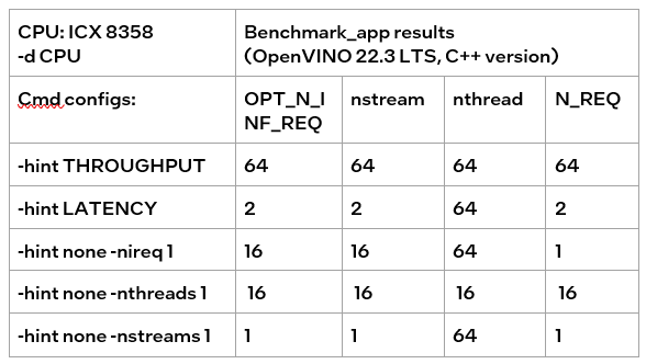
According to the results of the table, it can be obtained:
If only nireq is set, then nstreams and nthreads will be automatically set by the system according to HW. 64 threads are in the same NUMA node. CPU cores are evenly distributed between execution streams (every 4 threads). nstreams =64/4=16. For the first time, it is recommended not to set nireq. By setting other parameters of benchmark_app, the Optimal Number of Inference Requests can be obtained, which can be used as a reference for further tuning.
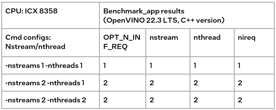
The max value of nthreads depends on the physical core. Setting nthreads alone doesn't make sense. Further tests set two of nireq, nstreams and nthreads at the same time, and the results are listed in the table below.
According to the table, when setting thread and stream simultaneously, there should be more nthreads than the nthreads. Otherwise, the default nthreads is equal to nthreads. The nthreads setting here is equivalent to binding hardware resources for the stream. This operation is implemented in the OpenVINO runtime. Users familiar with Linux may use other methods outside OpenVINO to bind hardware resources, namely numactl. As discussed before, this method is not suitable for VPS. Although not recommended, the following sections analyze the use of numactl on bare metal servers.
Tip3:
numactl is equivalent to the low-level settings on a bare metal server. Ensure the consistency of numactl and low-level settings, when using simultaneously.
The premise is to use numactl correctly, that is, use it on the same socket.
Evaluation: Low-level setting vs numactl
The numactl has been introduced above, and the usage is directly shown here.
numactl-C 0,1 . /benchmark_app -m ‘path to your model’ -hint none -nstreams 1-nthreads 1
Note:
"-C" refers to the CPUs you want to bind. You can check the numa node through “numactl–hardware”.
The actual CPU operation can be monitored through the htop tool.
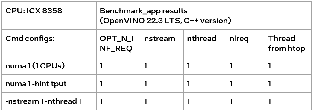
We could find out that using numactl alone or with the high-level hint is equivalent to the low-level settings. This shows that the principle of binding cores is the same. Although numactl can easily bind the core without any settings, it cannot change the ratio between nstreams and nthreads.
In addition, when numactl and the low-level setting are used simultaneously, the inconsistent settings will cause problems.
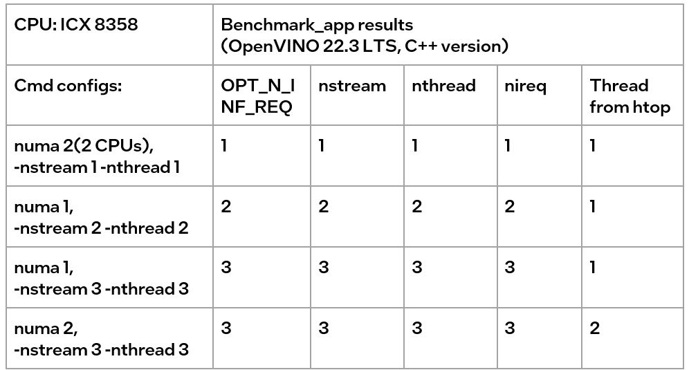
We can find the following results, according to the data in the table
- When the number of CPUs (set by NUMA) > nthread, determined by nthread, Benchmark_app results are equal to the number of CPUs monitored by htop
- When the number of CPUs (set by NUMA) < nthread, htop monitors that the number of CPUs is equal to the number controlled by NUMA, but an error message appears in Benchmark_app results, and the latency is exactly equal to the multiple of nstream.
The reason is that numactl is a global control, and benchmark_app can’t be corrected, resulting in latency equal to the result of repeated operations. The printed result is inconsistent with the actual monitoring, meaningless.
Summary:
Tip 1: For initial model testing on VPS, it is recommended to use the high-level settings of Python version Benchmark_app without numactl directly.
Tip 2: To balance the performance and hardware requirement on the bare metal server, a Low-level setting without numactl for the CPU is recommended, always set the nstreams first and tune with nthreads.
Tip 3: numactl is equivalent to the low-level settings on a bare metal server. Ensure the consistency of numactl and low-level setting, when using simultaneously.
Enable OpenVINO™ Optimization for WeNet
Introduction
The WeNet model provides two-pass approach to unify streaming and non-streaming end-to-end (E2E) speech recognition which is widely used with various HW platforms. In this blog, we provide the OpenVINO™ optimization for WeNet on Intel® platforms.
The public WeNet project is referenced from: wenet-e2e/wenet
The WeNet model can be considered as a pipeline which is split into 3 parts for decoder, CTC and encoder. Refer the model structure in below picture:

We implement the wrapper function of Automatic Speech Recognition (ASR) model class with OpenVINO™ runtime API programming for these 3 models’ data preparation and inference. Please refer the integrated OpenVINO™ optimization in official project: wenet-e2e/wenet/runtime/openvino
OpenVINO™backend on WeNet
In this project, you do not require to download OpenVINO™ and build the library with WeNet project manually. It’s already fully integrated with OpenVINO™ runtime library for downloading, program compiling and linking. If your operating system is not one of OpenVINO™ runtime library supported, the script will download OpenVINO™ source from Github, and build with CPU plugin to support.
At present, this repository already optimized and validated by OpenVINO™ 2022.3.0 version. Check the operating system which can support OpenVINO™ runtime library directly:
- Windows* 10
- CentOS 7, Red Hat* Enterprise Linux* 8
- Ubuntu* 18.04, 20.04
- Debian 9.13 for X86
- macOS* 10.15
Step 1: Get pretrained ONNX model (Optional)
If you already have the exported ONNX model for WeNet test, you can skip this step.
For users to get pretrained model from WeNet project, you can refer this link:
https://github.com/wenet-e2e/wenet/blob/main/docs/pretrained_models.en.md
Export to 3 ONNX models, including encoder.onnx, ctc.onnx and decoder.onnx by export_onnx_cpu script.
Step 2: Convert ONNX model to OpenVINO™ Intermediate Representation (IR)
Make sure your python environment already installed OpenVINO™ runtime library.
Convert these three ONNX models into IR by OpenVINO™ Model Optimizer command:
Step 3: Build WeNet with OpenVINO™ backend
Please refer system requirement to check if the hardware platform available by OpenVINO™. It will download and install OpenVINO™ library during the CMake configuration.
Some users may cannot easily download OpenVINO™ binary package from server due to firewall or proxy issue. If you failed to download by CMake script, you can download OpenVINO™ package by your selves and put the package to below path:
If you already have OpenVINO™ runtime which is manually built before the WeNet building, you can put the runtime library to below path:
Step 4: Simple inference test
You may run the inference test like below with the speech input audio file (.wav) and model unit file (.txt):
The information of OpenVINO™ integration and results will be print out:
Techniques for faster AI inference throughput with OpenVINO on Intel GPUs
Authors: Mingyu Kim, Vladimir Paramuzov, Nico Galoppo
Intel’s newest GPUs, such as Intel® Data Center GPU Flex Series, and Intel® Arc™ GPU, introduce a range of new hardware features that benefit AI workloads. Starting with the 2022.3 release, OpenVINO™ can take advantage of two newly introduced hardware features: XMX (Xe Matrix Extension) and parallel stream execution. This article explains what those features are and how you can check whether they are enabled in your environment. We also show how to benefit from them with OpenVINO, and the performance impact of doing so.
What is XMX (Xe Matrix Extension)?
XMX is a hardware acceleration for matrix multiplication on the newest Intel™ GPUs. Given the same number of Xe Cores, XMX technology provides 4-8x more multiplication capacity at the same precision [1]. OpenVINO, powered by OneDNN, can take advantage of XMX hardware by accelerating int8 and fp16 inference. It brings performance gains in compute-intensive deep learning primitives such as convolution and matrix multiplication.
Under the hood, XMX is a well-known hardware architecture called a systolic array. Systolic arrays increase computational capacity without increasing memory (or register) access. The magic happens by pipelining multiple computations with a single data access, as opposed to the traditional fetch-compute-store pipeline. It is implemented by connecting multiple computation nodes in series. Data is fed into the front, goes through several steps of multiplication-add, and finally is stored back to memory.
How to check whether you have XMX?
You can check whether your GPU hardware (and software stack) supports XMX with OpenVINO™’s hello_query_device sample. When you run the sample application, it lists all detected inference devices along with its properties. You can check for XMX support by looking at the OPTIMIZATION_CAPABILITIES property and checking for the GPU_HW_MATMUL value.
In the listing below you can see that our system has two GPU devices for inference, and only GPU.1 has XMX support.
As mentioned, XMX provides a way to get significantly more compute capacity on a GPU. The next feature doesn’t provide more capacity, but it allows ways to use that capacity more efficiently.
What is parallel execution of multiple streams?
Another improvement of Intel®’s discrete GPUs is to process multiple compute streams in parallel. Certain deep learning inference workloads are too small to fill all hardware compute resources of a given GPU. In such a case it is beneficial to run multiple compute streams (or inference requests) in parallel, such that the GPU hardware has more work to process at any given point in time. With parallel execution of multiple streams, Intel GPUs can increase hardware efficiency.
How to check for parallel execution support?
As of the OpenVINO 2022.3 release, there is only an indirect way to query how many streams your GPU can process in parallel. In the next release it will be possible to query the range of streams using the ov::range_for_streams property query and the hello_query_device_sample. Meanwhile, one can use the benchmark_app to report the default number of streams (NUM_STREAMS). If the GPU does not support parallel stream execution, NUM_STREAMS will be 2. If the GPU does support it, NUM_STREAMS will be larger than 2. The benchmark_app log below shows that GPU.1 supports 4-stream parallel execution.
However, it depends on application usage
Parallel stream execution can bring significant performance benefit, but only when used appropriately by the application. It will bring good performance gain if the application can run multiple independent inference requests in parallel, whether from single process or multiple processes. On the other hand, if there is no opportunity for parallel execution of multiple inference requests, then there is no gain to be had from multi-stream hardware execution.
Demonstration of performance tuning through benchmark_app
DISCLAIMER: The performance may vary depending on the system and usage.
OpenVINO benchmark_app is a very handy tool to analyze performance in various conditions. Here we’ll show the performance trend for an Intel® discrete GPU with XMX and four parallel hardware execution streams.
The performance was measured on a pre-production version of the Intel® Arc™ A770 Limited Edition GPU with 16 GiB of memory. The host system is a 12th Gen Intel(R) Core(TM) i9-12900K with 64GiB of RAM (4 DDR4-2667 modules) running Ubuntu OS 20.04.5 LTS with Linux kernel 5.15.47.
Performance comparison with high-level performance hints
Even though all supported devices in OpenVINO™ offer low-level performance settings, utilizing them is not recommended outside of very few cases. The preferred way to configure performance in OpenVINO Runtime is using performance hints. This is a future-proof solution fully compatible with the automatic device selection inference mode and designed with portability in mind.
OpenVINO benchmark_app exposes the high-level performance hints with the performance hint option for easy configuration of best latency and throughput. In short, latency mode picks the optimal configuration for low latency with the cost of low throughput, and throughput mode picks the optimal configuration for high throughput with the cost of high latency.
The table below shows throughput for various combinations of execution configuration for resnet-50.
Throughput mode is achieving much higher FPS compared to latency mode because inference happens with higher batch size and parallel stream execution. You can also see that, in throughput mode, the throughput with fp16 is 5.4x higher than with fp32 due to the use of XMX.
In the experiments below we manually explore different configurations of the performance parameters for demonstration purposes; It is generally not recommended to tune manually. Once the optimal parameters are known, they can be applied in production.
Performance gain from XMX
Performance gain from XMX can be observed by comparing int8/fp16 against fp32 performance because OpenVINO does not provide an option to turn XMX off. Since fp32 computations are not executed by the XMX hardware pipe, but rather by the less efficient fetch-compute-store pipe, you can see that the performance gap between fp32 and fp16 is much larger than the expected factor of two.
We choose a batch size of 64 to demonstrate the best case performance gain. When the batch size is small, the performance difference is not always as prominent since the workload could become too small for the GPU.
As you can see from the execution log, fp16 runs ~5.49x faster than fp32. Int8 throughput is ~2.07x higher than fp16. The difference between fp16 and fp32 is due to fp16 acceleration from XMX while fp32 is not using XMX. The performance gain of int8 over fp16 is 2.07x because both are accelerated with XMX.
Performance gain from parallel stream execution
You can see from the log below that performance goes up as we have more streams up to 4. It is because the GPU can handle 4 streams in parallel.
Note that if the inference workload is large enough, more streams might not bring much or any performance gain. For example, when increasing the batch size, throughput may saturate earlier than at 4 streams.
How to take advantage the improvements in your application
For XMX, all you need to do is run your int8 or fp16 model with the OpenVINO™ Runtime version 2022.3 or above. If the model is fp32(single precision), it will not be accelerated by XMX. To quantize a model and create an OpenVINO int8 IR, please refer to Quantizing Models Post-training. To create an OpenVINO fp16 IR from a fp32 floating-point model, please refer to Compressing a Model to FP16 page.
For parallel stream execution, you can set throughput hint as described in Optimizing for Throughput. It will automatically set the number of parallel streams with best number.
Conclusion
In this article, we introduced two key features of Intel®’s discrete GPUs: XMX and parallel stream execution. Most int8/fp16 deep learning networks can benefit from the XMX engine with no additional configuration. When properly configured by the application, parallel stream execution can bring significant performance gains too!
[1] In the Xe-HPG architecture, the XMX delivers 256 INT8 ops per clock (DPAS), while the (non-systolic) Xe Core vector engine delivers 64 INT8 ops per clock – a 4x throughput increase [reference]. In the Xe-HPC architecture, the XMX systolic array depth has been increased to 8 and delivers 4096 FP16 ops per clock, while the (non-systolic) Xe Core vector engine delivers 512 FP16 ops per clock – a 8x throughput increase [reference].
Notices & Disclaimers
Performance varies by use, configuration and other factors. Learn more at www.Intel.com/PerformanceIndex.
Performance results are based on testing as of dates shown in configurations and may not reflect all publicly available updates. See backup for configuration details. No product or component can be absolutely secure.
See backup for configuration details. For more complete information about performance and benchmark results, visit www.intel.com/benchmarks
© Intel Corporation. Intel, the Intel logo, and other Intel marks are trademarks of Intel Corporation or its subsidiaries. Other names and brands may be claimed as the property of others.

