

OpenVINO Blog

Running OpenVINO C++ samples on Visual Studio
Introduction
The OpenVINO™ samples provide practical examples of console applications developed in C, C++, and Python. These samples demonstrate how to leverage the capabilities of the OpenVINO API within your own applications. In this tutorial, we will guide you through the process of building and running the Hello Classification C++ Sample on Windows Visual Studio 2019 with OpenVINO 2023.0 release using Inception (GoogleNet) V3 deep learning model. The following steps outline the process:
Step 1: Install OpenVINO
Step 2: Download and Convert the Model
Step 3: Build OpenVINO C++ Runtime Samples
Step 4: Open the Solution and Run the Sample
Requirements
Before getting started, ensure that you have the following requirements in place:
- Microsoft Windows 10 or higher
- Microsoft Visual Studio 2019
- CMake version 3.10 or higher
Step 1: Install OpenVINO
To get started, you need to install OpenVINO Runtime C++ API and OpenVINO Development tools.
Download and Setup OpenVINO Runtime archive file for Windows.
- Download and extract the downloaded archive file to your local Downloads folder.
- Rename the extracted folder to “openvino_2023.0”
- Move the renamed folder to the “C:\Program Files (x86)\Intel” directory
- The "C:\Program Files (x86)\Intel\openvino_2023.0" folder now contains the core components for OpenVINO.
Configure the OpenVINO environment:
- Open the Windows Command Prompt.
- Run the following command to temporarily set OpenVINO environment variables. Please note that “setupvars.bat” works correctly only for Command Prompt, not for PowerShell.
Step 2: Download and Convert the Model
To successfully execute the "hello_classification” sample, a pre-trained classification model is required. You can choose a pre-trained classification model from either public models or Intel’s pre-trained models from the OpenVINO Open Model Zoo. However, before using these models in the "hello_classification" sample, they need to be downloaded and converted into the Intermediate Representation (IR) format using the Open Model Zoo tools. Following are the steps to install the tools and obtain the IR for the Inception (GoogleNet) V3 PyTorch model:
- Install OpenVINO Development Tools which include the necessary components for utilizing the Open Model Zoo Tools.
NOTE: Ensure that you install the same version of OpenVINO Development Tools as the OpenVINO Runtime C++ API. For more details, see these instructions.
- Next, execute the following commands to download and convert the googlenet-v3-pytorch model as an example:
NOTE: The googlenet-v3-pytorch IR files will be located at:
CURRENT_DIRECTORY\public\googlenet-v3-pytorch\FP32
Or you can specify the location of the model using:
Step 3: Build OpenVINO C++ Runtime Samples:
To build the OpenVINO C++ Runtime samples, follow these steps:
- In the existing Command Prompt where OpenVINO environment is setup, navigate to the "C:\Program Files (x86)\Intel\openvino_2022.3\samples\cpp" directory.
- Run the build_samples_msvc.bat script. By default, the script automatically detects the Microsoft Visual Studio installed on the machine and uses it to create and build a solution.
Step 4: Open the Solution and Run the Sample.
To open and run the Hello Classification sample in Visual Studio, follow these steps:
- Start the Visual Studio using Command Prompt:
- In Visual Studio, choose "Open a project or solution" from the menu and navigate to the following solution file:
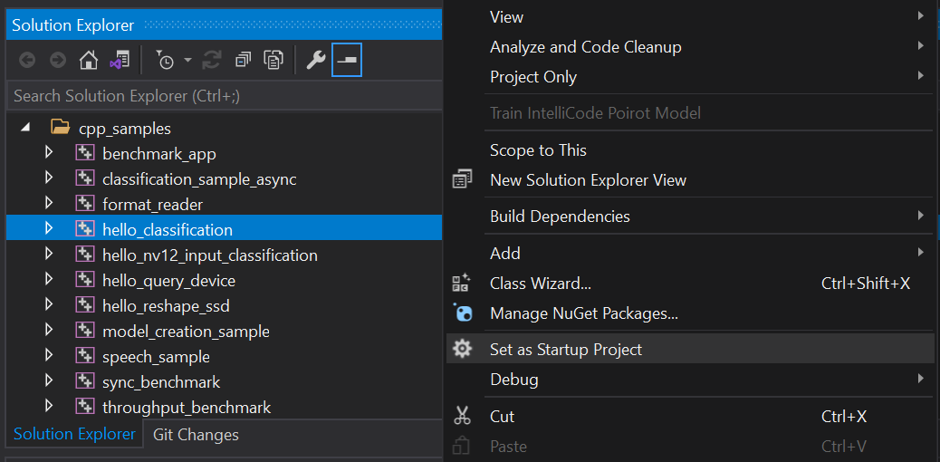
- Set the "hello_classification" project as the startup project (see Figure 1).
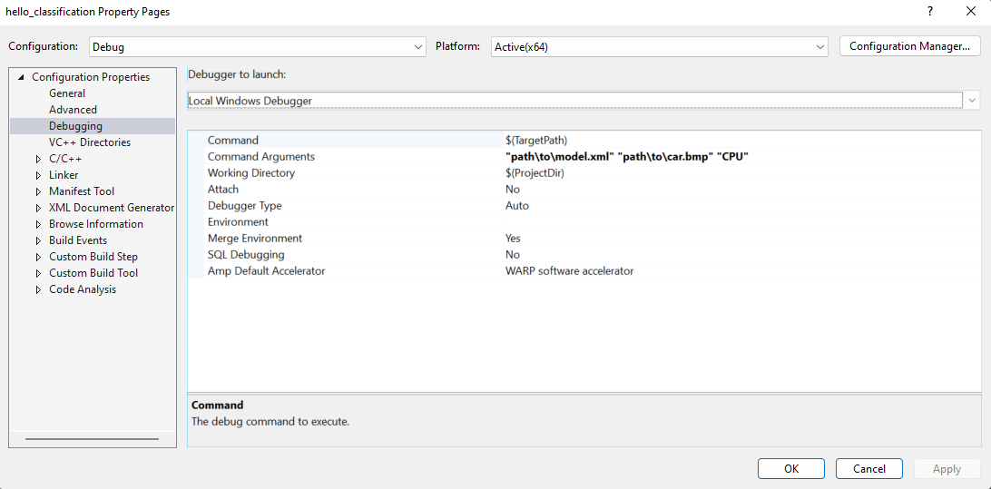
- To run the sample, you need to specify a model and image:
- Navigate to: project properties->Configuration properties->Debugging->Command Arguments
- Add command line arguments for the path to model, path to input image and device name (see Figure 2).
- You can use images from the media files collection available at test_data
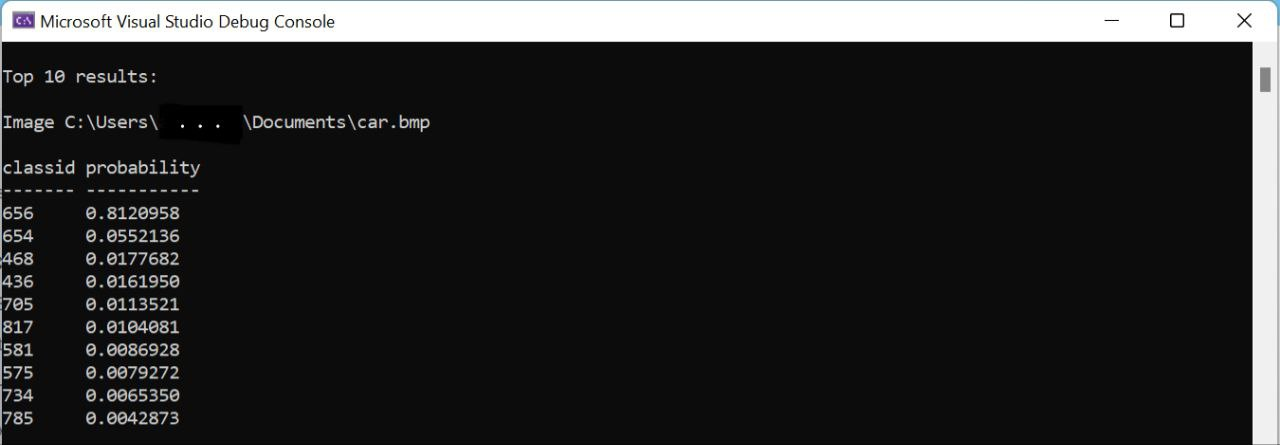
- Apply the changes and run the application. The application will output the top-10 inference results (see Figure 3).
Additional Resources:
For more information and detailed instructions, refer to the following resources:
OpenVINO™ Frontend Extension Samples with ConversionExtension
Authors: Wenyi Zou, Su Yang
The OpenVINO™ Frontend extension API enables the mapping of custom operations from framework model representation to OpenVINO representation. In this blog, two samples focus on the mapping to multiple operations with the ConversionExtension in practice.
Sample One: grid_sampler
This sample explains how to use Frontend ConversionExtension classes to facilitate the mapping of custom operations from ONNX model representation to OpenVINO™ representation. It enables writing arbitrary code to replace a single framework operation with multiple connected OpenVINO™ operations constructing dependency graph of any complexity.
When convert the ONNX model BEVFormer tiny to OpenVINO IR, the following error will occur.

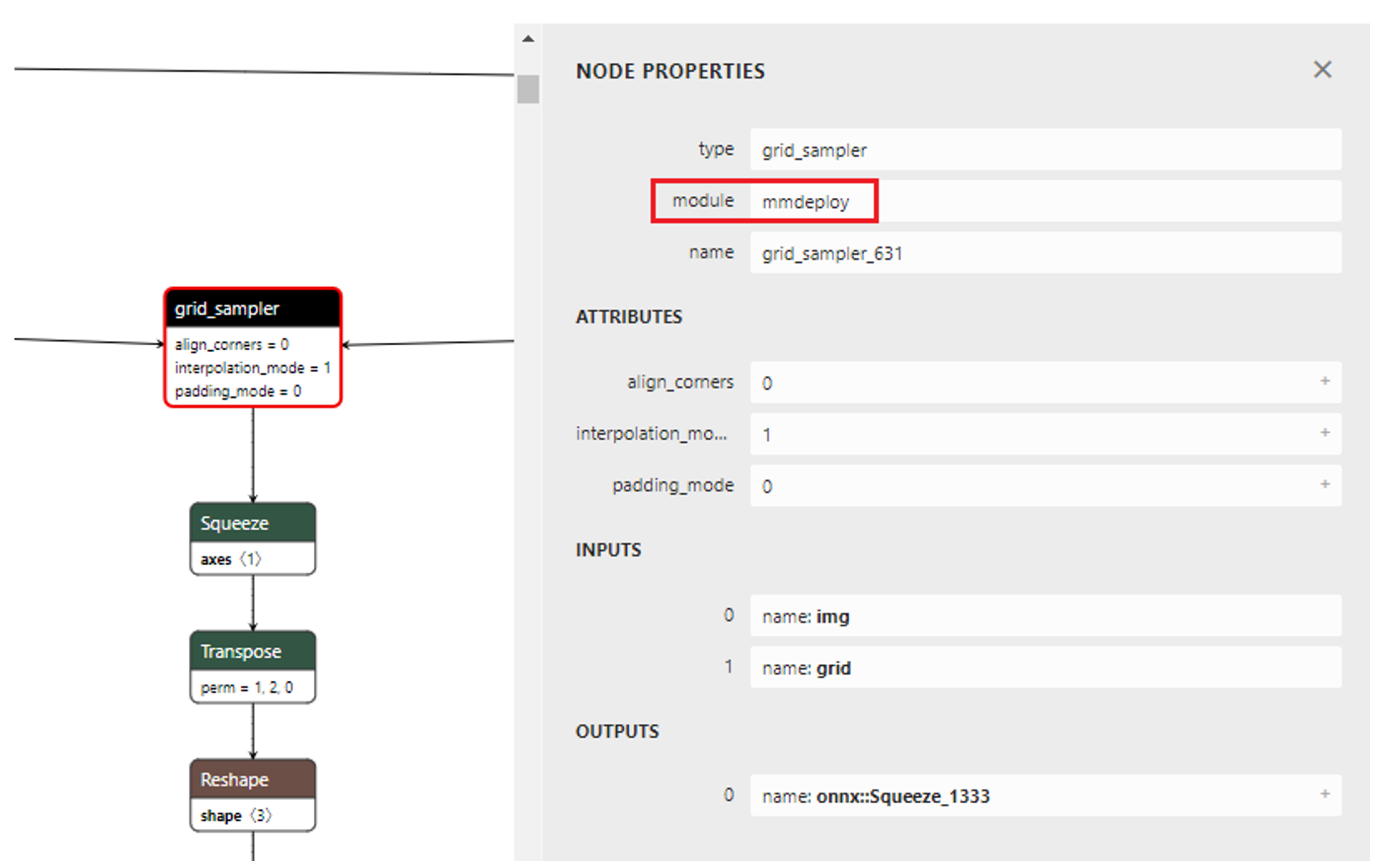
Network BEVFormer tiny viewing with Netron, we can see the node of grid_sampler. As shown in Figure 1.1.
ONNX Nodes
Computation nodes are comprised of a name, the name of an operator that it invokes, a list of named inputs, a list of named outputs, and a list of attributes.
Input and outputs are positionally associated with operator inputs and outputs. Attributes are associated with operator attributes by name.
They have the following properties:
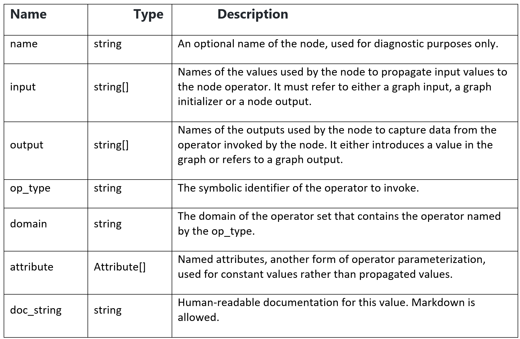
According to the node properties of ONNX, the node grid_sampler_631 op_type is grid_sampler, the domain is mmdeploy. We can use ov::frontend::onnx::ConversionExtension to set the domain paramerter.
Sample Two: aten::uniform
In the OpenVINO™ documentation, the example illustrates basic knowledge of ConversionExtension, like node object of type NodeContext. Real mapping issues like different node modules(or domains), different input types, and missing attributes are under discussion and solved with the workaround.
To support the VectorNet model, try to export the ONNX model from PyTorch. Unfortunately, aten::uniform (ATen is PyTorch’s built-in tensor library) isn’t yet supported by onnx. But OpenVINO™ has RandomUniform operation. Comparing the PyTorch Uniform operation with the RandomUniform operation (generates random numbers from a uniform distribution in the range [minval, maxval)), it shows the same math task with the different input types. Therefore, It’s possible to use Frontend Extensions to map this uniform distribution operation with the onnx model if solving the potential mapping issues. As one-to-one mapping is impossible, decomposition to multiple operations (at least Op Convert additionally) should be considered.
Export Model with Fallback
Because support has not been added to convert a particular torch op to ONNX, we cannot export each ATen op (in the TorchScript namespace “aten”) as a regular ONNX op. So, we fall back to exporting an ATen op with OperatorExportTypes.ONNX_ATEN_FALLBACK.
To optimize the onnx model with OpenVINO™ , create a new sample based on the C++ hello_classification in Linux.
Error: Check 'unknown_operators.empty()' failed at src/frontends/onnx/frontend/src/core/graph.cpp:213: OpenVINO™ does not support the following ONNX operations: org.pytorch.aten.Aten.
Visualize Graph for Mapping
In Netron, we could find 6 ATen nodes with the same input values. The obvious mapping problem is that the attribute uniform of node aten should be the node type, while the additional node’s domain is org.pytorch.aten. So, we use ov::frontend::onnx::conversion to set domain parameter, which is similar to the sample one.
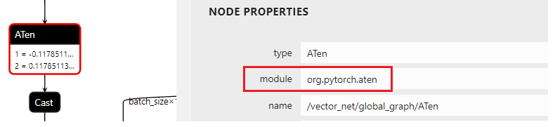
As below, real attributes of PyTorch uniform operation aren’t available in the ONNX. The needed attributes of OpenVINO™ RandomUniform operation are output_type, global_seed, and op_seed.
Note: Types are int32 or int64, while uniform op is float64 in the figure.
As a workaround, we set the seed of attributes as a constant because of the missing aten::uniform attributes.
To solve the difference between aten::uniform and RandomUniform, the mapping issue could be solved as below:
- Use Op ShapeOf to get the 1D tensor of the input shape.
- Use Op Convert to convert the input types from aten::uniform’s f64 to RandomUniform’s i64.
- Use Op Add the input with the Op Constant “117” and Op Multiply with the Op Constant “0.001”, because the output value of the upstream Op ConstantOfShape_output_0 is “0” and the real inputs of all six aten::uniform’s “minval” and “maxval” are “-0.11785113…” and “0.11785113…”.
Add Extension in Practice
Debug steps of the Frontend extension on Windows Visual Studio:
- Add add_extension code into C++ sample and build project
- Debug with onnx file path
Thanks to the NODE_VALIDATION_CHECK from random_uniform Op, the debug is friendly to the new user.
Code sample of the core.add_extension function
See Also
Reduce OpenVINO Model Server Latency with In-Process C-API
Starting with the 2022.3 release, OpenVINO Model Server (OVMS) provides a C-API that allows OVMS to be linked directly into a C/C++ application as a dynamic library. Existing AI applications can leverage serving functionalities while running inference locally without networking latency overhead.
The ability to bypass gRPC/REST endpoints and send input data directly from in-process memory creates new opportunities to use OpenVINO locally while maintaining the benefits of model serving. For example, we can combine the benefits of using OpenVINO Runtime with model configuration, version management and support for both local and cloud model storage.
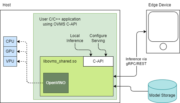
OpenVINO Model Server is typically started as a separate process or run in a container where the client application communicates over a network connection. Now, as you can see above, it is possible to link the model server as a shared library inside the client application and use the internal C API to execute internal inference methods.
We demonstrate the concept in a simple example below and show the impact on latency.
Example C-API Usage
NOTE: complete end to end inference demonstration via C-API with example app can be found here: https://docs.openvino.ai/latest/ovms_demo_capi_inference_demo.html
To start using the Model Server C-API, we need to prepare a model and configuration file. Download an example dummy model from our GitHub repo and prepare a config.json file to serve this model. “Dummy” model adds value 1 to all numbers inside an input.
Download Model
Create Config File
Get libovms_shared.so
Next, download and unpack the OVMS library. The library can be obtained from GitHub release page. There are 2 packages – one for Ubuntu 20 and one for RedHat 8.7. There is also documentation showing how to build the library from source. For purpose of this demo, we will use the Ubuntu version:
Start Server
To start the server, use ServerStartFromConfigurationFile. There are many options, all of which are documented in the header file. Let’s launch the server with configuration file and optional log level error:
Input Data Preparation
Use OVMS_InferenceRequestInputSetData call, to provide input data with no additional copy operation. In InferenceRequestNew call, we can specify model name (the same as defined in config.json) and specific version (or 0 to use default). We also need to pass input names, data precision and shape information. In the example we provide 10 subsequent floating-point numbers, starting from 0.
Invoke Synchronous Inference
Simply call OVMS_Inference. This is required to pass response pointer and receive results in the next steps.
Read Results
Use call OVMS_InferenceResponseGetOutput API call to read the results. There are bunch of metadata we can read optionally, such as: precision, shape, buffer type and device ID. The expected output after addition should be:
Check the header file to learn more about the supported methods and their parameters.
Compile and Run Application
In this example we omitted error handling and resource cleanup upon failure. Please refer to the full demo instructions for a more complete example.
Performance Analysis
Using benchmarking tools from OpenVINO Runtime and both the C-API and gRPC API in OpenVINO Model Server, we can compare inference results via C-API to typical scenario of gRPC or direct integration of OpenVINO Runtime. The Resnet-50-tf model from Open Model Zoo was used for the testing below.
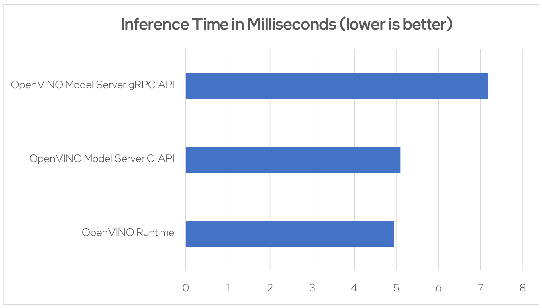
Hardware configuration used:
- 1-node, Intel Xeon Gold 6252 @ 2.10GHz processor with 256GB (8 slots/16GB/2666) total DDR memory, HT on, Turbo on, Ubuntu 20.04.2 LTS,5.4.0-109-generic kernel
- Intel S2600WFT motherboard
Tested by Intel on 01/31/2023.
Conclusion
With the new method of embedding OVMS into C++ applications, users can decrease inference latency even further by entirely skipping the networking part of model serving. The C-API is still in preview and has some limitations, but in its current state is ready to integrate into C++ applications. If you have questions or feedback, please file an issue on GitHub.
Read more:
- Complete API description: https://docs.openvino.ai/latest/ovms_docs_c_api.html
- End to end demo: https://docs.openvino.ai/latest/ovms_demo_capi_inference_demo.html
OpenVINO optimizer Latent Diffusion Models (LDM) for super-resolution
OpenVINO optimizer Latent Diffusion Models(LDM) for super-resolution
Introduction
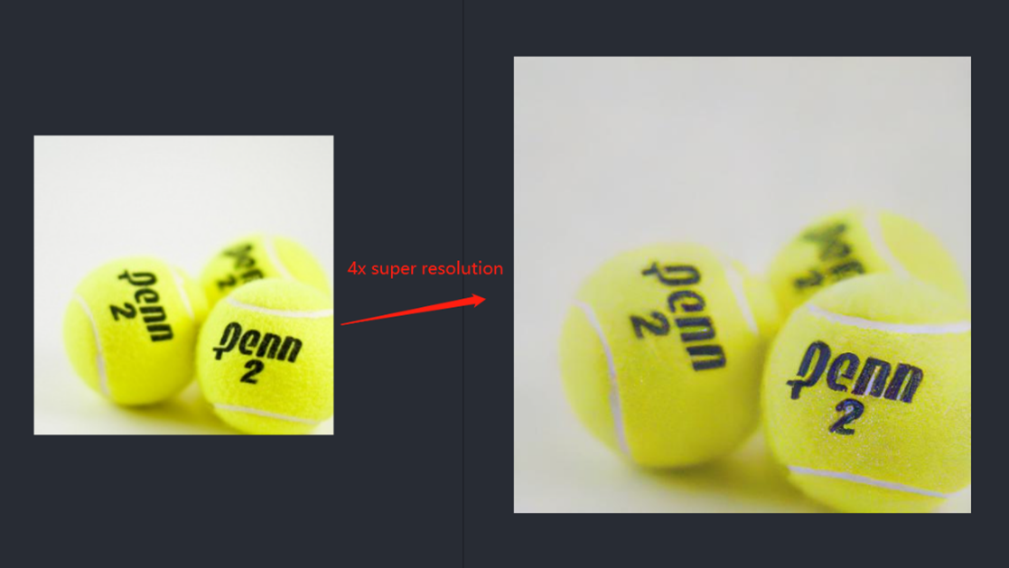
A computer vision approach called image super-resolution aims to increase the resolution of low-resolution images so that they are clearer and more detailed. Applicationsfor super-resolution include the processing of medical images, surveillancefootage, and satellite images.
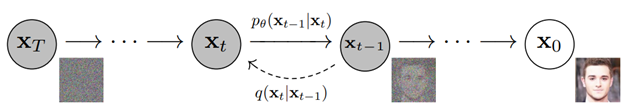
The LDM (LatentDiffusion Models) Super Resolution model, a deep learning-based approach to photo super-resolution, was developed by the Hugging Face Research team. The residual network (ResNet) architecture, a type of convolutional neural network(CNN) created to address the issue of vanishing gradients in deep neuralnetworks.
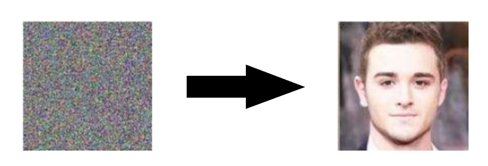
Diffusion models are generative models,meaning that they are used to generate data similar to the data on which they are trained. Fundamentally, Diffusion Models work by destroying training data through the successive addition of Gaussian noise, andthen learning to recover the data by reversing this noising process. After training, we can use the Diffusion Model to generatedata by simply passing randomly sampled noise through the learned denoising process.
Diffusion Model is a latent variable model which maps to the latent space using a fixed Markov chain. This chain gradually adds noise to thedata in order to obtain the approximate posterior.
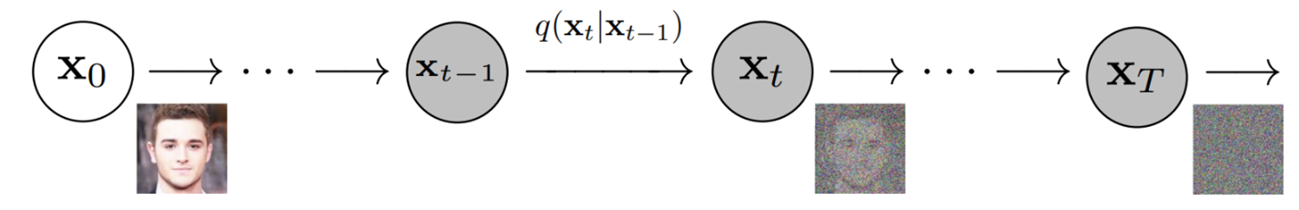
Ultimately, the image is asymptotically transformed to pure Gaussian noise. The goal of training a diffusion model is to learn the reverse process. By traversing backward along this chain, we can generate new data.
Requirement
- Optimum-intel Optimum Intel is the interface betweenthe HuggingFace Transformers and Diffusers libraries and the differenttools and libraries provided by Intel to accelerate end-to-end pipelines onIntel architectures.
Intel Neural Compressor is an open-source library enabling the usageof the most popular compression techniques such as quantization, pruning and knowledge distillation
- OpenVINO™ is an open-sourcetoolkit for optimizing and deploying AI inference which can boost deep learningperformance in computer vision, automatic speech recognition, natural language processing and other common task.
- optimum-intel==1.5.2(include openvino)
- openvino
- openvino-dev
- diffusers
- pytorch >= 1.9.1
- onnx >= 1.13.0
Reference: optimum-intel-ldm-super-resolution-4x
QuickStart Demo
Original repo is from HuggingFace CompVis/ldm-super-resolution-4x-openimages,we are reference to build our pipeline to implement super-resolution related function.
To transformand acceleration optimize the pipeline by openvino, there are 3 steps need to do.
- Step1. Install the requirement package and initial environment.
- Step2. Convert original model to openvino IR model.
- Step3. Build OpenVINO super resolution pipeline.
Now, Let’s start with the content of our tutorial.
Step 1. Install the requirementpackage and initial environment
OpenVINO has the standard installation process, we can directly refer tothe official OpenVINO documentation to install.
Reference: Install OpenVINO by source code for Linux
Reference: Install OpenVINO by release package
Optimum Intel also can refer the standard guide.
Reference: Optimum-intel install guide
(Optional) Install the latest stable release by pipe :
# pip install openvino, openvino-dev
# pip install"optimum[openvino,nncf]"
Step 2. Convert originalmodel to OpenVINO IR model
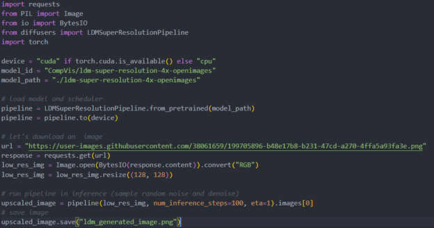
Firstly, run pipe the HuggingFace pipeline, it will automate download the models, and we need to convert them from pytorch->onnx->IR, to enable the model by OpenVINO.
%20workflow.png)
The LDM (LatentDiffusion Models) Super Resolution model has two part of sub-models: unet and vqvae,we should convert each of them in to IR model.
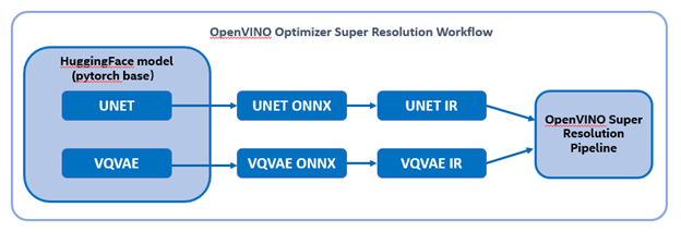
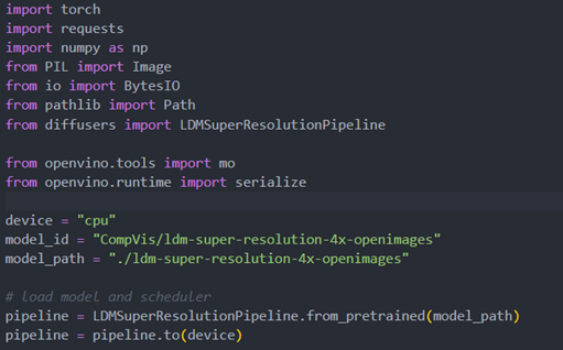
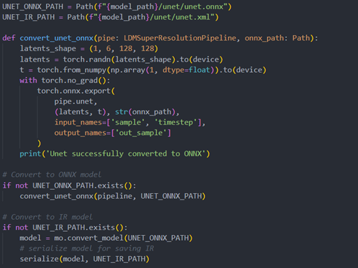
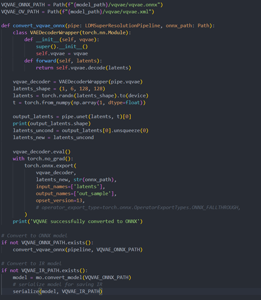
The reference source code for model convert,also we provide the script in the GitHub repo : ov-ldm4x-model-convert.py
Initial parameter and the ov-pipeline
Unet sub-model convert to IR
Vqvae sub-model convert to IR
Step 3. Build OpenVINOsuper resolution pipeline
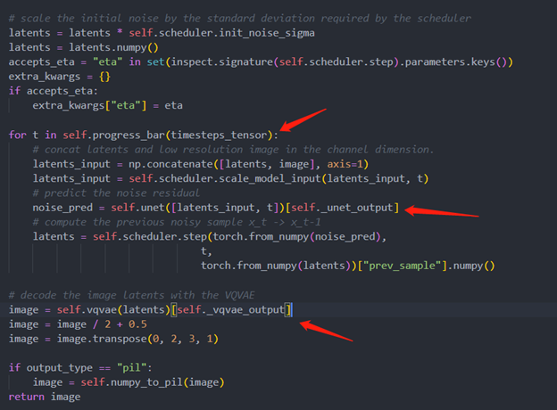
The LDM (Latent Diffusion Models) Super Resolution OpenVINO pipeline main function part code, the whole pipeline script is provided in GitHub repo: ov-ldm4x-pipeline.py
Inference Result
Deploy End to End Super-Resolution Pipeline with OpenVINO™ Model Server
Introduction
In this blog, we will show how to deploy an end-to-end super-resolution pipeline by leveraging OpenVINOTM Model Server with Demultiplexing in DAG and Custom Node features.
OpenVINOTM Model Server (OVMS) is a high-performance system for serving models that uses the same architecture and API as TensorFlow Serving and KServe while applying OpenVINOTM for inference execution. It is implemented in C++ for scalability and optimized for deployment on intel architectures.
Directed Acyclic Graph (DAG) is an OVMS feature that controls the execution of an entire graph of interconnected models defined within the OVMS configuration. The DAG scheduler makes it possible to create a pipeline of models for execution in the server with a single client request.
During the pipeline execution, it is possible to split a request with multiple batches into a set of branches with a single batch. Internally, OVMS demultiplexer will divide the data, process them in parallel and combine the results.
The custom node in OVMS simplifies linking deep learning models into complete pipeline. Custom node can be used to implement all operations on the data which cannot be handled by the neural network model. It is represented by a C++ dynamic library implementing OVMS API defined in custom_node_interface.h.
Super-Resolution Pipeline Workflow
Figure1 shows the super-resolution pipeline in a flowchart, where we use "demultiply_counter=3" without loss of generality. The whole pipeline starts with input data from the Request node via gRPC calls. Batched input data with 5D shape(3,1,3,270,480) is split into a single batch by the DAG demultiplexer. Each single batch of data is fed into a custom node for image preprocessing. The two outputs of the custom node serve as inputs for model A inference. In the end, all inference results are gathered as output C, which will be sent by the Response node to the client via gRPC calls.
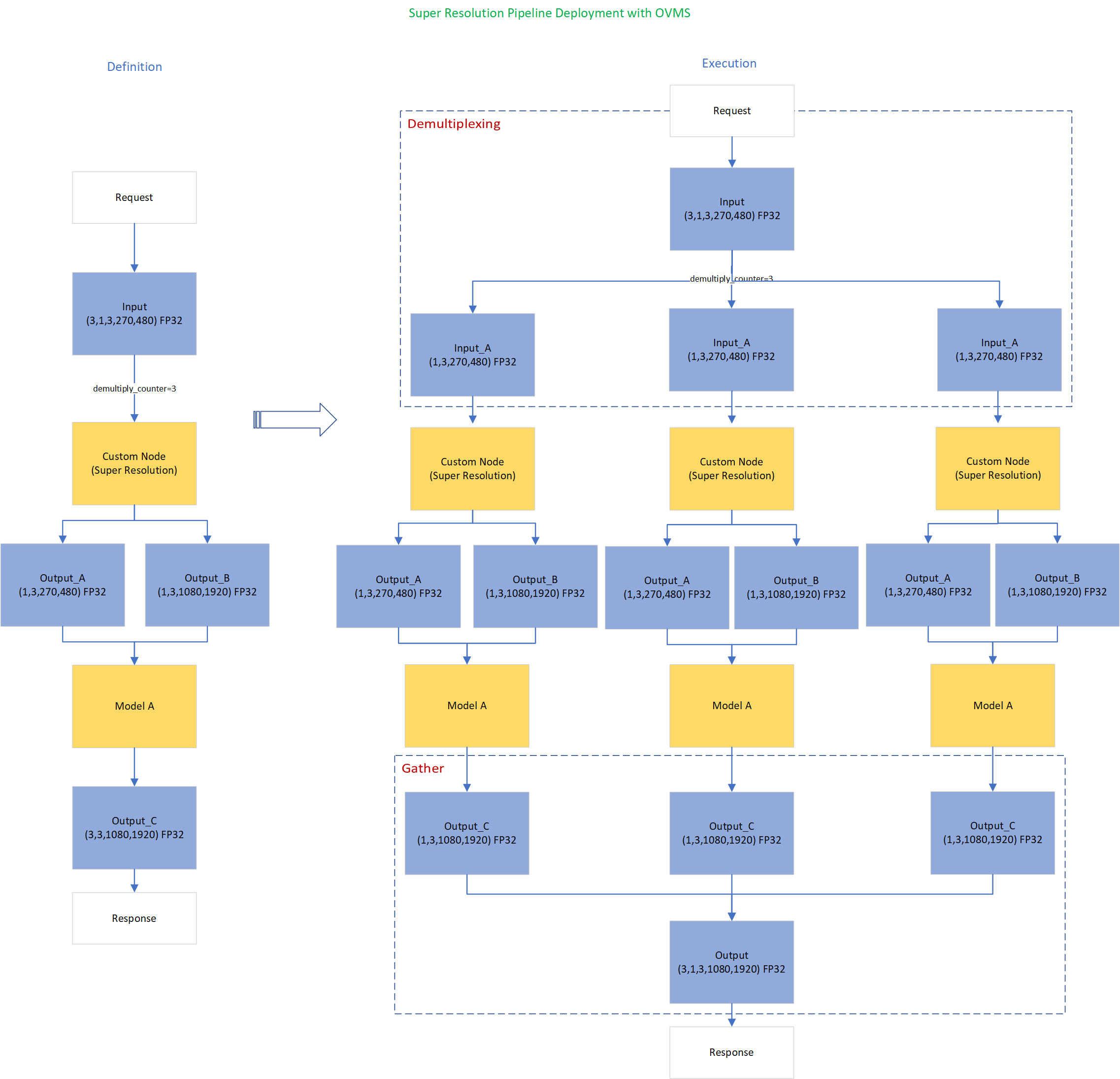
Here is an example configuration for the super-resolution pipeline deployed with OVMS.
“pipeline_config_list” contains super-resolution pipeline information, data enter from the “request” node, flow to “sr_preprocess_node” for image preprocessing, generated two outputs will serve as inputs in “super_resolution_node” for inference, gathered inference results will be returned by “response” node.
- "demultiply_count": acceptable input data batch size when Demultiplexing in DAG feature enabled, “demultiply_count” with value -1 means OVMS can accept dynamic batch input data.
“model_config_list”: contains the basic configuration for super-resolution deep learning model and OpenVINOTM CPU plugin configuration.
- "nireq": set number of infer requests used in OVMS server for deep learning model
- "NUM_STREAMS": set number of streams used in the CPU plugin
- "INFERENCE_PRECISION_HINT": option to select preferred inference precision in CPU plugin. We can set "INFERENCE_PRECISION_HINT":bf16 on the Xeon platform that supports BF16 precision, such as the 4th Gen Intel® Xeon® Scalable processor (formerly codenamed Sapphire Rapids). Otherwise, we should set "INFERENCE_PRECISION_HINT":f32 as the default value.
“custom_node_library_config_list”: contains the name and path of the custom node dynamic library
Image Preprocessing with libvips in Custom Node
In this blog, we use a single-image-super-resolution model from Open Model Zoo for the super-resolution pipeline. The model requires two inputs according to the model specification. The first input is the original image (shape [1,3,270,480]). The second input is a 4x resized image with bicubic interpolation (shape [1,3,1080,1920]). Both input images expected color space is BGR. Therefore, image preprocessing for input image is required.
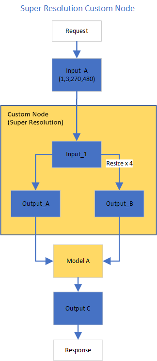
Figure2 shows the custom node designed for image preprocessing in the super-resolution pipeline. The custom node takes the original input image as input data. At first, input data is assigned to output 1 without modification. Besides, the input data is resized 4x with bicubic interpolation and assigned as output 2. The two outputs are passed to the model node for inference. For image processing in the custom node, we utilize libvips – an open-source image processing library that is designed to be fast and efficient with low memory usage. Please see the detailed custom node implementation in super_resolution_nhwc.cpp.
Although libvips is very sufficient for image processing operations with less memory, libvips does not provide functionality for layout (NCHW->NHWC) and color space (RGB->BGR) conversion, which is required by the super-resolution model as inputs. Instead, we can integrate layout and color space conversion into models using OpenVINOTM Preprocessing API.
Integrate Preprocessing with OpenVINOTM Preprocessing API
OpenVINOTM Preprocessing API allows adding custom preprocessing steps into the execution graph of OpenVINOTM models.
Here is a sample code to integrate layout (NCHW-> NHWC) and color space (BRG->RGB) conversion into the super-resolution model with OpenVINOTM Preprocessing API.
In the code snippet above, we first load the original model and initialize the PrePostProcessor object with the original model. Then we modify the model's 1st input element type to “uint8”, change the color format from the default “BGR” to “RGB”, and set the layout from “NCHW” to “NHWC”. In the end, we build a new model and serialize it on the disk. The whole model preprocessing can be done offline, please find details in model_preprocess.py.
Build Model Server Docker Image for Super-Resolution Pipeline
Build OVMS docker image with custom node
Copy compiled custom nodes library to the “models” directory
Setup client environment
Integrate preprocessing with OpenVINOTM Preprocessing API
The resulting model will be saved in the “super_resolution_model_preprocessed/1” directory.
Super-Resolution Pipeline Demo
Start the OpenVINOTM Model Server with docker binding with 8 cores
Run client with command line
Figure 3 shows the original input image (shape 270x480).

Figure 4 shows the resized image (shape 1080x1920) after image preprocessing in the custom node.

Figure 5 shows the inference result of the super-resolution model (shape1080x1920).

Conclusion
In this blog, we demonstrate an end-to-end super-resolution pipeline deployment with OpenVINOTM Model Server. The whole pipeline takes dynamic batched images (RGB, NHWC) as input, demultiplexing into single batch data, preprocess with a custom node, runs an inference with a super-resolution model, send gathered inference results to the client in the end.
This blog provides following examples that utilize OpenVINOTM Model Server and OpenVINOTM features:
- Enable OVMS DAG demultiplexing feature
- Provide custom node for image preprocessing using libvips
- Provide sample code for integrating preprocessing into the model with OpenVINOTM Preprocessing API.
- Support super-resolution end-to-end pipeline with image preprocessing and model inference with OVMS DAG scheduler
Remote Tensor API Sample
This AI pipeline implements zero-copy between SYCL and OpenVINO through the Remote Tensor API of the GPU Plugin.
- Introduction
The development of SYCL simplifies the use of OpenCL, which can fully exploit the computing power of GPU in the pipeline. Meanwhile, SYCL has more flexibility to do customized pre- and post-processing of OpenVINO. To further optimize the pipeline, developers can use GPU Plugin to avoid the memory copy overhead between SYCL and OpenVINO. The GPU plugin provides the ov::RemoteContext and ov::RemoteTensor interfaces for video memory sharing and interoperability with existing native APIs, such as OpenCL, Microsoft DirectX, or VAAPI. For details, please refer to the online documentation of OpenVINO.
Based on the pseudocode of the online documentation, here we provide a simple pipeline sample with Remote Tensor API. Because in the rapid iteration of oneAPI, sometimes customers need quick verification so that this sample can be used for testing. OneAPI also provides a real-world, end-to-end example, which optimizes PointPillars for lidar object detection.
- Components
SYCL preprocessing is based on the Sepia Filter sample, which demonstrates how to convert a color image to a Sepia tone image, a monochromatic image with a distinctive Brown Gray color. The sample program works by offloading the compute-intensive conversion of each pixel to Sepia tone using SYCL*-compliant code for CPU and GPU.
OpenVINO inferencing is based on the OpenVINO classification sample, the input from SYCL filtered image in the device will be sent into OpenVINO as a remote tensor without a memory copy.
Remote Tensor API: Create RemoteContext from SYCL pre-processing’s native handle. After model compiling, do memory sharing between the application and GPU plugin with from cl::Buffer to remote tensor.
- Build Sample on Linux
Download the source code from the link. Prepare the model and images.
To run the sample, you need to specify a model and image:
Use pre-trained models from the Open Model Zoo. The models can be downloaded using the Model Downloader. Use images from the media files collection.
Run on Intel NUC Core 11 iGPU with OpenVINO 2022.2 and oneAPI 2022.3.
./intel64/hello_nv12_input_classification_oneAPI../model/FP32/alexnet.xml ../image/dog512.bmp GPU 2
Sample Output:
Warning: With the updating of OpenVINO and oneAPI, different versions may cause problems with the tools in the common directory or the new SYCL header name. Please use the same version or debug following the corresponding release instructions.
Accelerate Inference of Sparse Transformer Models with OpenVINO™ and 4th Gen Intel® Xeon® Scalable Processors
Authors: Alexander Kozlov, Vui Seng Chua, Yujie Pan, Rajesh Poornachandran, Sreekanth Yalachigere, Dmitry Gorokhov, Nilesh Jain, Ravi Iyer, Yury Gorbachev
Introduction
When it comes to the inference of overparametrized Deep Neural Networks, perhaps, weight pruning is one of the most popular and promising techniques that is used to reduce model footprint, decrease the memory throughput required for inference, and finally improve performance. Since Language Models (LMs) are highly overparametrized and contain lots of MatMul operations with weights it looks natural to prune the redundant weights and benefit from sparsity at inference time. There are several types of pruning methods available:
- Fine-grained pruning (single weights).
- Coarse pruning: group-level pruning (groups of weights), vector pruning (rows in weights matrices), and filter pruning (filters in ConvNets).
Contemporary Language Models are basically represented by Transformer-based architectures. Using coarse pruning methods for such models is problematic because of the many connections between the layers. This trait means that, first, not every pruning type is applicable to such models and, second, pruning of some dimension in one layer requires adjustments in the rest of the layers connected to it.
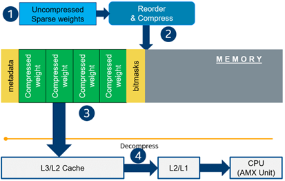
Fine-grained sparsity does not have such a constraint and can be applied to each layer independently. However, it requires special support on the HW and inference SW level to get real performance improvements from weight sparsity. There are two main approaches that help to leverage from weight sparsity at inference:
- Skip multiplication and addition for zero weights in dot products of weights and activations. This usually results in a special instruction set that implements such logic.
- Weights compression/decompression to reduce the memory throughput. Compression is performed at the model load/compilation stage while decompression happens on the fly right before the computation when weights are in the cache. Such a method can be implemented on the HW or SW level.
In this blog post, we focus on the SW weight decompression method and showcase the end-to-end workflow from model optimization to deployment with OpenVINO.
Sparsity support in OpenVINO
Starting from OpenVINO 2022.3release, OpenVINO runtime contains a feature that enables weights compression/decompression that can lead to performance improvement on the 4thGen Intel® Xeon® Scalable Processors. However, there are some prerequisites that should be considered to enable this feature during the model deployment:
- Currently, this feature is available only to MatMul operations with weights (Fully-connected layers). So currently, there is no support for sparse Convolutional layers or other operations.
- MatMul layers should contain a high level of weights sparsity, for example, 80% or higher which is achievable, especially for large Transformer models trained on simple tasks such as Text Classification.
- The deployment scenario should be memory-bound. For example, this prerequisite is applicable to cloud deployment when there are multiple containers running inference of the same model in parallel and competing for the same RAM and CPU resources.
The first two prerequisites assume that the model is pruned using special optimization methods designed to introduce sparsity in weight matrices. It is worth noting that pruning methods require model fine-tuning on the target dataset in order to reduce accuracy degradation caused by zeroing out weights within the model. It assumes the availability of the HW capable of DL model training. Nowadays, many frameworks and libraries offer such methods. For example, PyTorch provides some capabilities for NN pruning. There are also resources that offer pre-trained sparse models that can be used as a starting point, for example, SparseZoo from Neural Magic.
OpenVINO also provides instruments for DL model pruning implemented in Neural Network Compression Framework (NNCF) that is aimed specifically for model optimization and offers different optimization options: from post-training optimization to deep compression when stacking several optimization methods. NNCF is also integrated into Hugging Face Optimum library which is designed to optimize NLP models from Hugging Face Hub.
Using only sparsity is not so beneficial compared to another popular optimization method such as bit quantization which can guarantee better performance-accuracy trade-offs after optimization in the general case. However, the good thing about sparsity is that it can be stacked with 8-bit quantization so that the performance improvements of one method reinforce the optimization effect of another one leading to a higher cumulative speedup when applying both. Considering this, OpenVINO runtime provides an acceleration feature for sparse and 8-bit quantized models. The runtime flow is shown in the scheme below:
Below, we demonstrate two end-to-end workflows:
- Pruning and 8-bit quantization of the floating-point BERT model using Hugging Face Optimum and NNCF as an optimization backend.
- Quantization of sparse BERT model pruned with 3rd party optimization solution.
Both workflows end up with inference using OpenVINO API where we show how to turn on a runtime option that allows leveraging from sparse weights.
Pruning and 8-bit quantization with Hugging Face Optimum and NNCF
This flow assumes that there is a Transformer model coming from the Hugging Face Transformers library that is fine-tuned for a downstream task. In this example, we will consider the text classification problem, in particular the SST2 dataset from the GLUE benchmark, and the BERT-base model fine-tuned for it. To do the optimization, we used an Optimum-Intel library which contains the optimization capabilities based on the NNCF framework and is designed for inference with OpenVINO. You can find the exact characteristics and steps to reproduce the result in this model card on the Hugging Face Hub. The model is 80% sparse and 8-bit quantized.
To run a pre-optimized model you can use the following code from this notebook:
Quantization of already pruned model
In case if you deal with already pruned model, you can use Post-Training Quantization from the Optimum-Intel library to make it 8-bit quantized as well. The code snippet below shows how to quantize the sparse BERT model optimized for MNLI dataset using Neural Magic SW solution. This model is publicly available so that we download it using Optimum API and quantize on fly using calibration data from MNLI dataset. The code snippet below shows how to do that.
Enabling sparsity optimization inOpenVINO Runtime and 4th Gen Intel® Xeon® Scalable Processors
Once you get ready with the sparse quantized model you can use the latest advances of the OpenVINO runtime to speed up such models. The model compression feature is enabled in the runtime at the model compilation step using a special option called: “CPU_SPARSE_WEIGHTS_DECOMPRESSION_RATE”. Its value controls the minimum sparsity rate that MatMul operation should have to be optimized at inference time. This property is passed to the compile_model API as it is shown below:
An important note is that a high sparsity rate is required to see the performance benefit from this feature. And we note again that this feature is available only on the 4th Gen Intel® Xeon® Scalable Processors and it is basically for throughput-oriented scenarios. To simulate such a scenario, you can use the benchmark_app application supplied with OpenVINO distribution and limit the number of resources available for inference. Below we show the performance difference between the two runs sparsity optimization in the runtime:
- Benchmarking without sparsity optimization:
- Benchmarking when sparsity optimization is enabled:
Performance Results
We performed a benchmarking of our sparse and 8-bit quantized BERT model on 4th Gen Intel® Xeon® Scalable Processors with various settings. We ran two series of experiments where we vary the number of parallel threads and streams available for the asynchronous inference in the first experiments and we investigate how the sequence length impact the relative speedup in the second series of experiments.
The table below shows relative speedup for various combinations of number of streams and threads and at the fixed sequence length after enabling sparsity acceleration in the OpenVINO runtime.
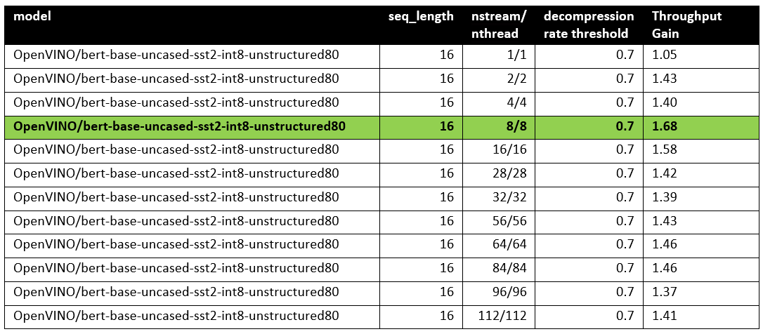
Based on this, we can conclude that one can expect significant performance improvement with any number of streams/threads larger than one. The optimal performance is achieved at eight streams/threads. However, we would like to note that this is model specific and depends on the model architecture and sparsity distribution.
The chart below also shows the relationship between the possible acceleration and the sequence length.
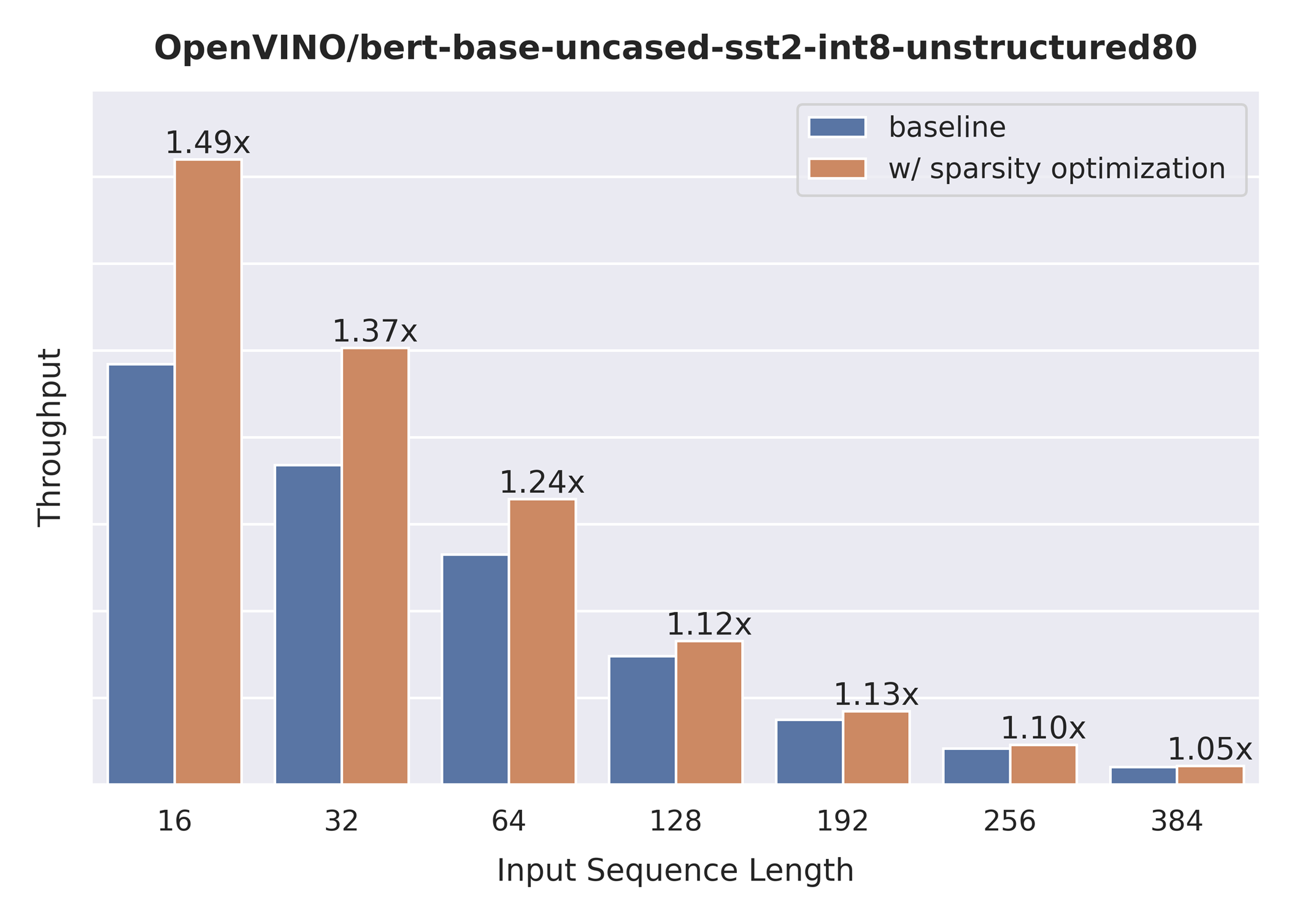
As you can see the benefit from sparsity is decreasing with the growth of the sequence length processed by the model. This effect can be explained by the fact that for larger sequence lengths the size of the weights is no longer a performance bottleneck and weight compression does not have so much impact on the inference time. It means that such a weight sparsity acceleration feature does not suit well for large text processing tasks but could be very helpful for Question Answering, Sequence Classification, and similar tasks.
References
OpenVINO™ Enable PaddlePaddle Quantized Model
OpenVINO™ is a toolkit that enables developers to deploy pre-trained deep learning models through a C++ or Python inference engine API. The latest OpenVINO™ has enabled the PaddlePaddle quantized model, which helps accelerate their deployment.
From floating-point model to quantized model in PaddlePaddle
Baidu releases a toolkit for PaddlePaddle model compression, named PaddleSlim. The quantization is a technique in PaddleSlim, which reduces redundancy by reducing full precision data to a fixed number so as to reduce model calculation complexity and improve model inference performance. To achieve quantization, PaddleSlim takes the following steps.
- Insert the quantize_linear and dequantize_linear nodes into the floating-point model.
- Calculate the scale and zero_point in each layer during the calibration process.
- Convert and export the floating-point model to quantized model according to the quantization parameters.
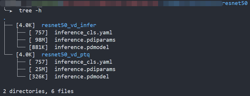
As the Figure1 shows, Compared to the floating-point model, the size of the quantized model is reduced by about 75%.
Enable PaddlePaddle quantized model in OpenVINO™
As the Figure2.1 shows, paired quantize_linear and dequantize_linear nodes appear intermittently in the model.
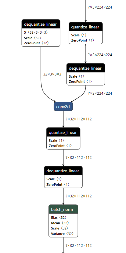
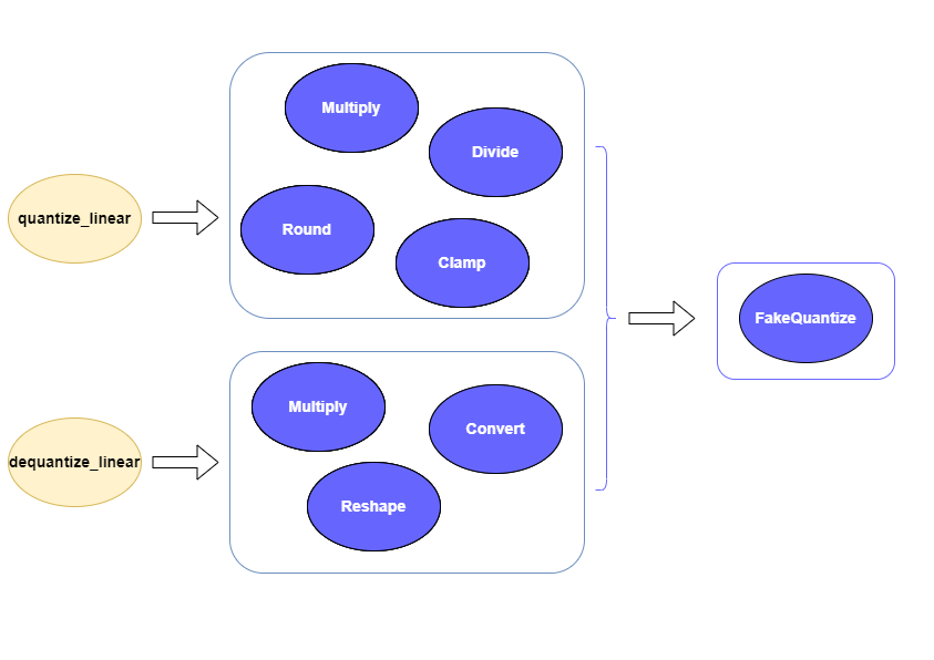
In order to enable PaddlePaddle quantized model, both quantize_linear and dequantize_linear nodes should be mapped first. And then, quantize_linear and dequantize_linear pattern scan be fused into FakeQuantize nodes and OpenVINO™ transformation mechanism will simplify and optimize the model graph in the quantization mode.
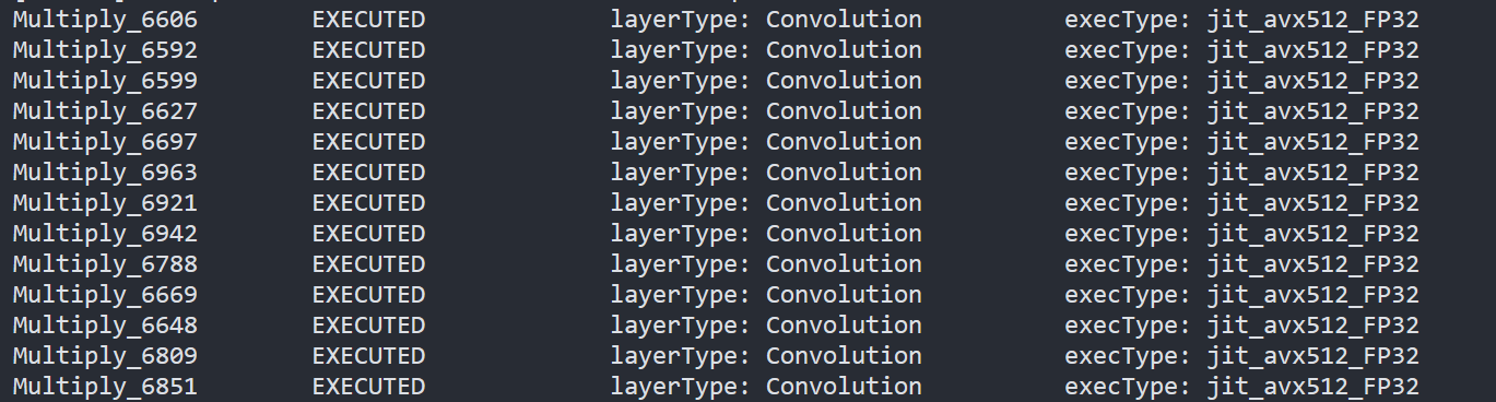
To check the kernel execution function, just profile and dump the execution progress, you can use benchmark_app as an example. The benchmark_app provides the option"-pc", which is used to report the performance counters information.
- To report the performance counters information of PaddlePaddle resnet50 float model, we can run the command line:
- To report the performance counters information of PaddlePaddle resnet50 quantized model, we can run the command line:
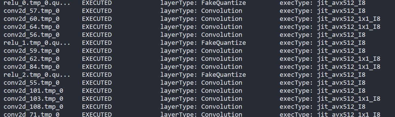
By comparing the Figure2.3 and Figure2.4, we can easily find that the hotpot layers of PaddlePaddle quantized model are dispatched to integer ISA implementation, which can accelerate the execution.
Accuracy
We compare the accuracy between resnet50 floating-point model and post training quantization(PaddleSlim PTQ) model. The accuracy of PaddlePaddle quantized model only decreases slightly, which is expected.
Performance
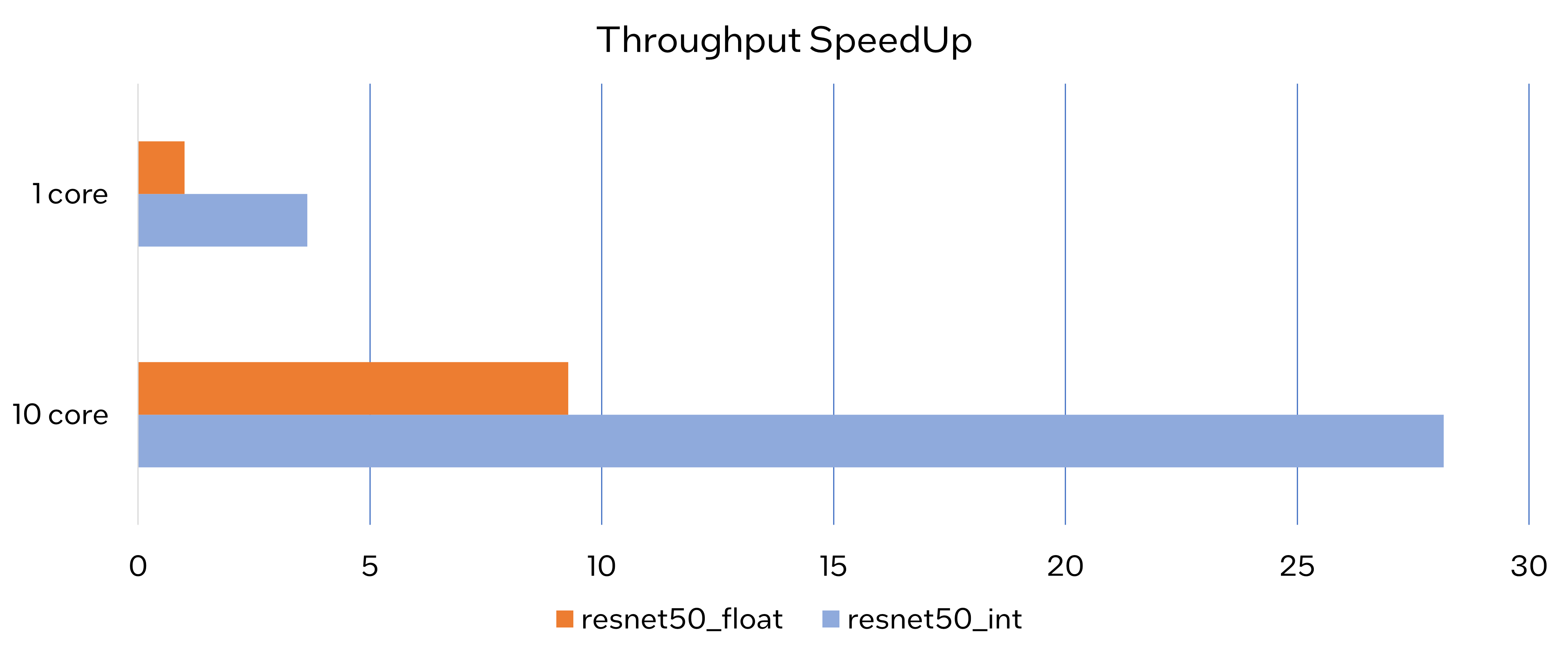
Throughput Speedup
The throughput of PaddlePaddle quantized resnet50 model can improve >3x.
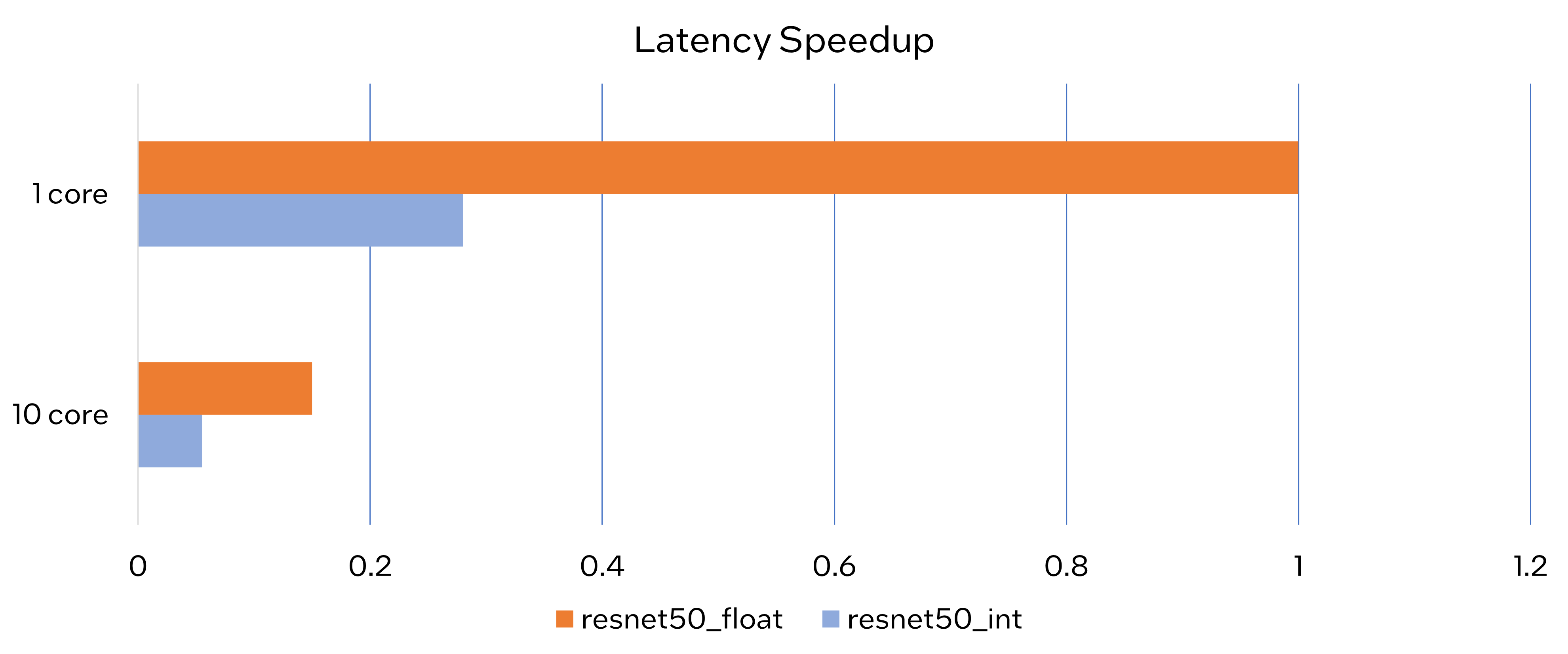
Latency Speedup
The latency of PaddlePaddle quantized resnet50 model can reduce about 70%.
Conclusion
In this article, we elaborated the PaddlePaddle quantized model in OpenVINO™ and profiled the accuracy and performance. By enabling the PaddlePaddle quantized model in OpenVINO™, customers can accelerate both throughput and latency of deployment easily.
Notices & Disclaimers
- The accuracy data is collected based on 50000 images of val dataset in ILSVRC2012.
- The throughput performance data is collected by benchmark_app with data_shape "[1,3,224,224]" and hint throughput.
- The latency performance data is collected by benchmark_app with data_shape "[1,3,224,224]" and hint latency.
- The machine is Intel® Xeon® Gold 6346 CPU @3.10GHz.
- PaddlePaddle quantized model can be achieve at https://github.com/PaddlePaddle/FastDeploy/blob/develop/docs/en/quantize.md.