

OpenVINO Blog

OpenVINO GenAI Serving (OGS)
Authors: Fiona Zhao, Xiake Sun, Wenyi Zou, Su Yang, Tianmeng Chen
Model Server reference implementation based on OpenVINO GenAI Package for Edge/Client AI PC Use Case.
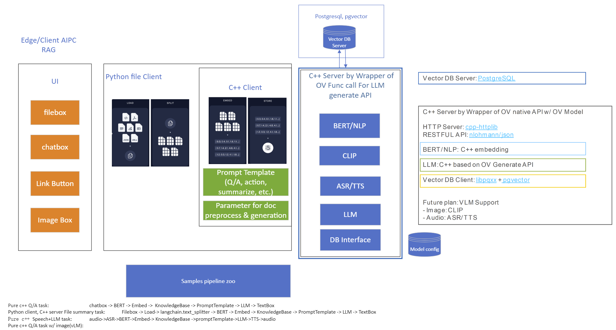
Use Case 1: C++ RAG Sample that supports most popular models like LLaMA 2
This example showcases for Retrieval-Augmented Generation based on text-generation Large Language Models (LLMs): chatglm, LLaMA, Qwen and other models with the same signature and Bert model for embedding feature extraction. The sample fearures ov::genai::LLMPipeline and configures it for the chat scenario. There is also a Jupyter notebook which provides an example of LLM-powered RAG in Python.
Download and convert the model and tokenizers
The --upgrade-strategy eager option is needed to ensure optimum-intel is upgraded to the latest version.
Setup of PostgreSQL, Libpqxx and Pgvector
Langchain's document Loader and Spliter
- Load: document_loaders is used to load document data.
- Split: text_splitter breaks large Documents into smaller chunks. This is useful both for indexing data and for passing it in to a model, since large chunks are harder to search over and won’t in a model’s finite context window.
PostgreSQL
Download postgresql from enterprisedb.(postgresql-16.2-1-windows-x64.exe is tested)
Install PostgreSQL with postgresqltutorial.
Setup of PostgreSQL:
1. Open pgAdmin 4 from Windows Search Bar.
2. Click Browser (left side) > Servers > Postgre SQL 10.
3. Create the user postgres with password openvino (or your own setting)
4. Open SQL Shell from Windows Search Bar to check this setup. 'Enter' to set Server, Database, Port, Username as default and type Password.
libpqxx
'Official' C++ client library (language binding), built on top of C library
Update the source code from https://github.com/jtv/libpqxx in deps\libpqxx
The pipeline connects with DB based on Libpqxx.
pgvector
Open-source vector similarity search for Postgres.
By default, pgvector performs exact nearest neighbor search, which provides perfect recall. It also supports approximate nearest neighbor search (HNSW), which trades some recall for speed.
For Windows, Ensure C++ support in Visual Studio 2022 is installed, then use nmake to build in Command Prompt for VS 2022(run as Administrator). Please follow with the pgvector
Enable the extension (do this once in each database where you want to use it), run SQL Shell from Windows Search Bar with "CREATE EXTENSION vector;".
Printing CREATE EXTENSION shows successful setup of Pgvector.
pgvector-cpp
pgvector support for C++ (supports libpqxx). The headers (pqxx.hpp, vector.hpp, halfvec.hpp) are copied into the local folder rag_sample\include. Our pipeline does the vector similarity search for the chunks embeddings in PostgreSQL, based on pgvector-cpp.
Install OpenVINO, VS2022 and Build this pipeline
Download 2024.2 release from OpenVINO™ archives*. This OV built package is for C++ OpenVINO pipeline, no need to build the source code. Install latest Visual Studio 2022 Community for the C++ dependencies and LLM C++ pipeline editing.
Extract the zip file in any location and set the environment variables with dragging this setupvars.bat in the terminal Command Prompt. setupvars.ps1 is used for terminal PowerShell. <INSTALL_DIR> below refers to the extraction location. Run the following CMD in the terminal Command Prompt.
Notice:
- Install on Windows: Copy all the DLL files of PostgreSQL, OpenVINO and tbb and openvino-genai into the release folder. The SQL DLL files locate in the installed PostgreSQL path like "C:\Program Files\PostgreSQL\16\bin".
- If cmake not installed in the terminal Command Prompt, please use the terminal Developer Command Prompt for VS 2022 instead.
- The openvino tokenizer in the third party needs several minutes to build. Set 8 for -j option to specify the number of parallel jobs.
- Once the cmake finishes, check rag_sample_client.exe and rag_sample_server.exe in the relative path .\build\samples\cpp\rag_sample\Release.
- If Cmake completed without errors, but not find exe, please open the .\build\OpenVINOGenAI.sln in VS2022, and set the solution configuration as Release instead of Debug, then build the llm project within VS2022 again.
Run
Launch RAG Server
rag_sample_server.exe --llm_model_path TinyLlama-1.1B-Chat-v1.0 --llm_device CPU --embedding_model_path bge-large-zh-v1.5 --embedding_device CPU --db_connection "user=postgres host=localhost password=openvino port=5432 dbname=postgres"
Lanuch RAG Client
rag_sample_client.exe
Lanuch python Client
Use python client to send the message of DB init and send the document chunks to DB for embedding and storing.
python client_get_chunks_embeddings.py --docs test_document_README.md
Enable ControlNet with Stable Diffusion Pipeline via Optimum-Intel
Authors: Tianmeng Chen, Xiake Sun
Introduction
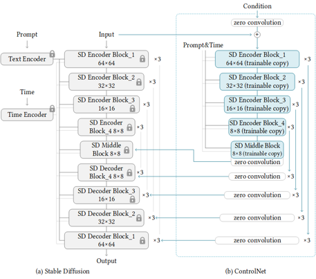
Stable Diffusion is a generative artificial intelligence model that produces unique images from text and image prompts. ControlNet is a neural network that controls image generation in Stable Diffusion by adding extra conditions. The specific structure of Stable Diffusion + ControlNet is shown below:
In many cases, ControlNet is used in conjunction with other models or frameworks, such as OpenPose, Canny, Line Art, Depth, etc. An example of Stable Diffusion + ControlNet + OpenPose:
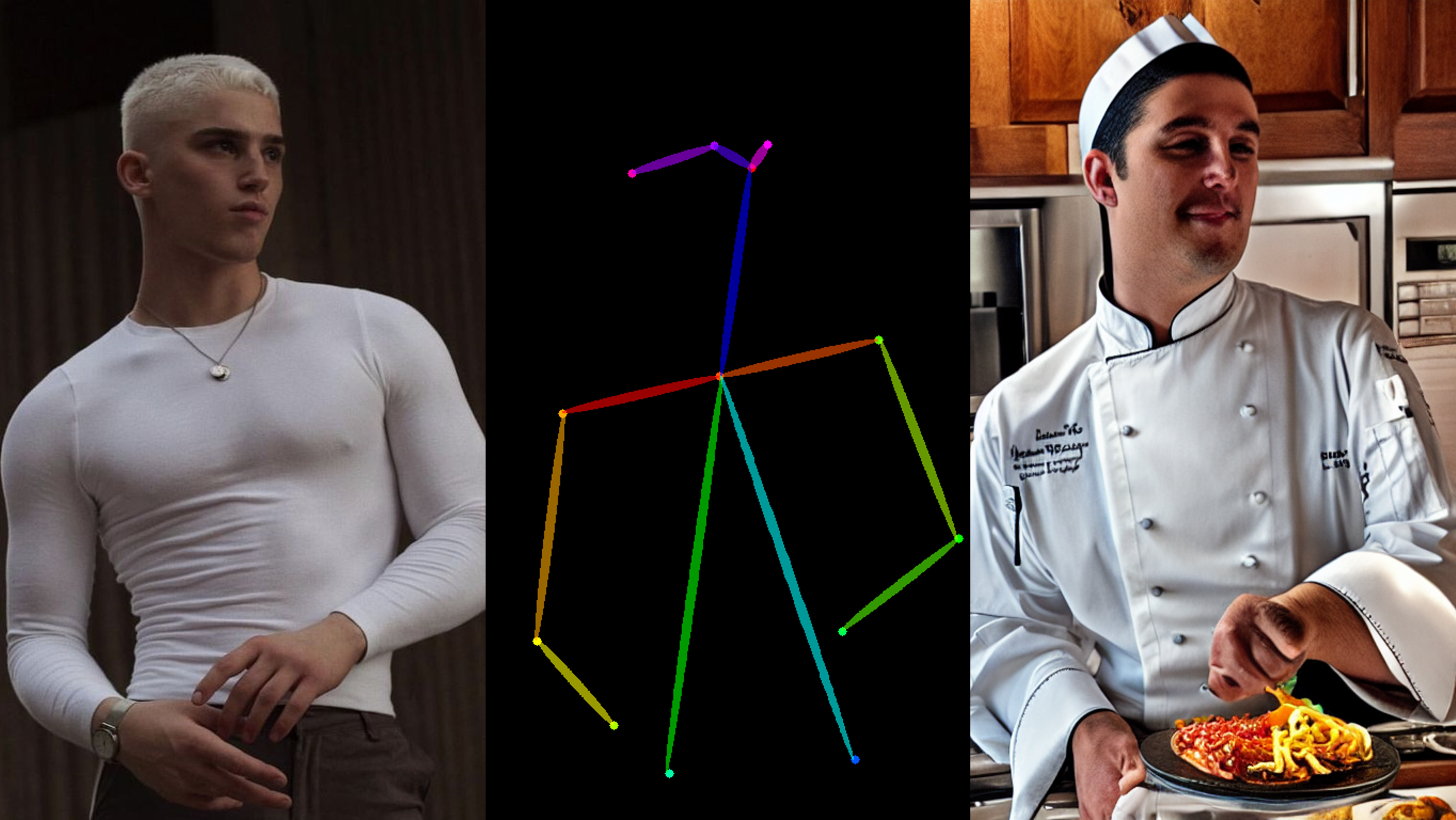
OpenPose identifies the key points of the human body from the left image to get the pose image, and then inputs the Pose image to ControlNet and Stable Diffusion to get the right image. In this way, ControlNet can control the generation of Stable Diffusion.
In this blog, we focus on enabling the stable diffusion pipeline with ControlNet in Optimum-intel. Some details can be found in this open PR.
How to enable StableDiffusionControlNet pipeline in Optimum-Intel
The important code is in optimum/intel/openvino/modelling_diffusion.py and optimum/exporters/openvino/model_configs.py. There is the diffusion pipeline related code in file modelling_diffusion.py, you can find several Class: OVStableDiffusionPipelineBase, OVStableDiffusionPipeline, OVStableDiffusionXLPipelineBase, OVStableDiffusionXLPipeline, and so on. What we need to do is mimic these base classes to add the OVStableDiffusionControlNetPipelineBase, StableDiffusionContrlNetPipelineMixin, and OVStableDiffusionControlNetPipeline. A few of the important parts are as follows:
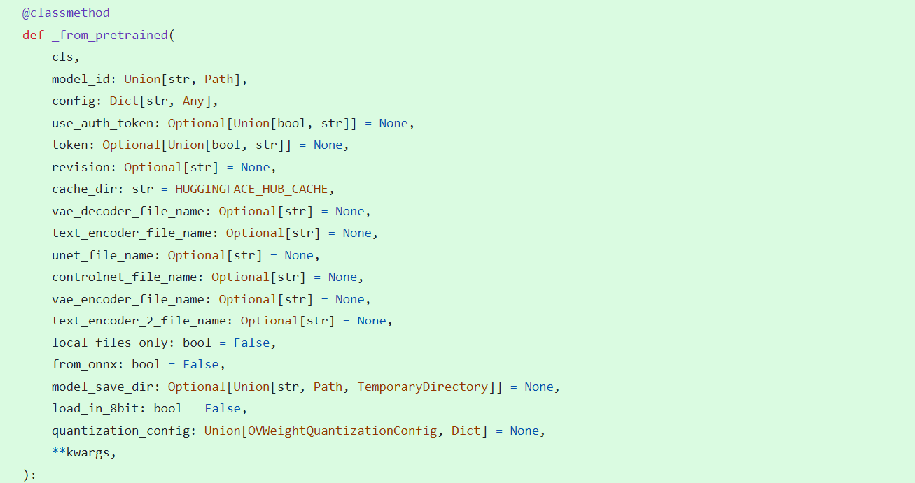
_from_pretrained function in class OVStableDiffusionControlNetPipelineBase: initial whole pipeline from local or download.
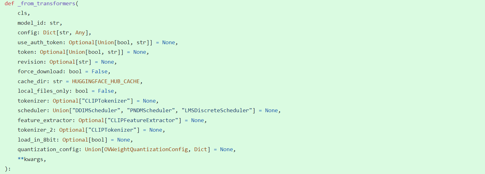
_from_transformers function in class OVStableDiffusionControlNetPipelineBase: convert torch model to OpenVINO IR model.
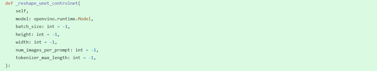
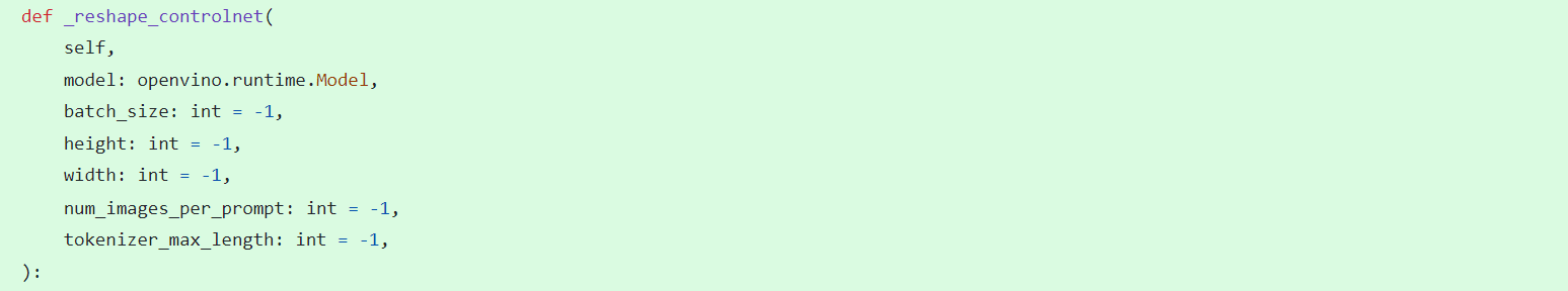
_reshape_unet_controlnet and _reshape_controlnet in class OVStableDiffusionControlNetPipelineBase: reshape dynamic OpenVINO IR model to static in order to decrease cost.
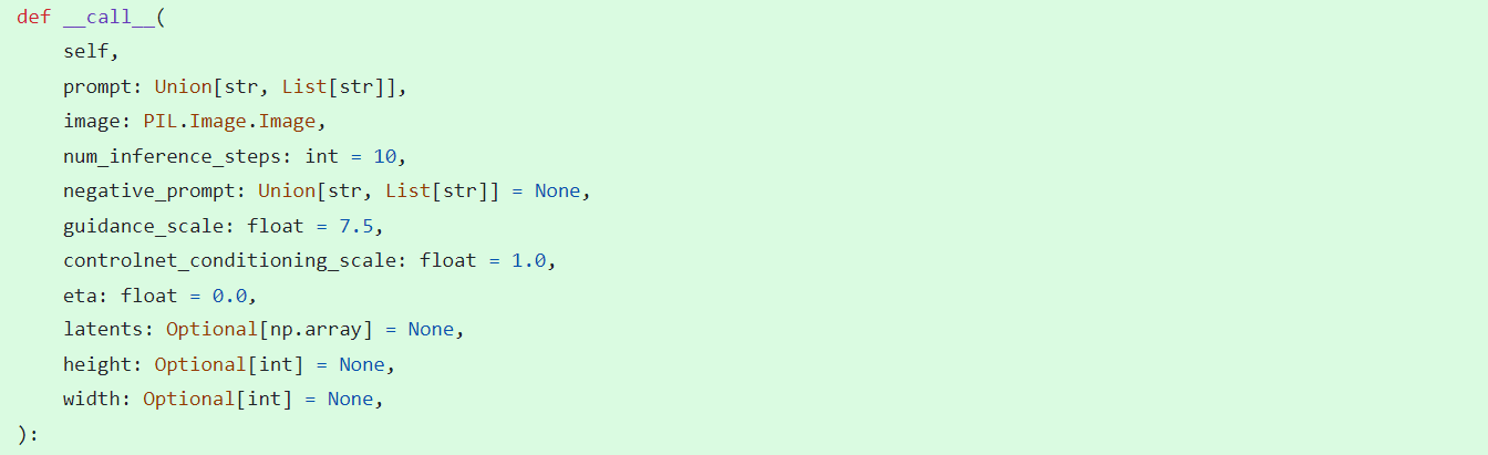
__call__ function in class StableDiffusionContrlNetPipelineMixin: do the inference in the pipeline.
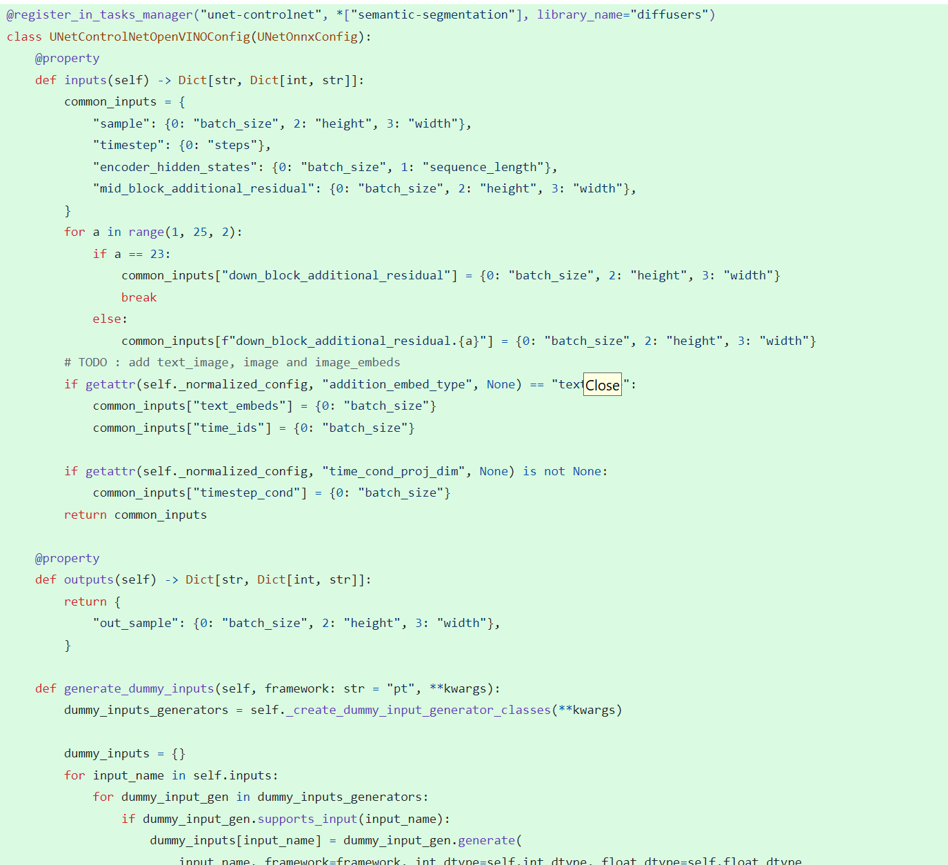
In model_configs.py, we define UNetControlNetOpenVINOConfig by inheriting UNetOnnxConfig, which includes UNetControlNet inputs and outputs.
By now we have completed the rough code, after which some very detailed code additions are needed, so I won't go into that here.
How to use StableDiffusionControlNet pipeline via Optimum-Intel
The next step is how to use the code, examples of which can be found in this repository.
Installation and update of environments and dependencies from source. Make sure your python version is greater that 3.10 and your optimum-intel and optimum version is up to date accounding to the requirements.txt.
# %python -m venv stable-diffusion-controlnet
# %source stable-diffusion-controlnet/bin/activate
%pip install -r requirements.txt
At first, we should convert pytorch model to openvino IR with dynamic shape. Now import related packages.
from optimum.intel import OVStableDiffusionControlNetPipeline
import os
from diffusers import UniPCMultistepScheduler
Set pytroch models of stable diffusion 1.5 and controlnet path if you have them in local, else you can run pipeline from download.
SD15_PYTORCH_MODEL_DIR="stable-diffusion-v1-5"
CONTROLNET_PYTORCH_MODEL_DIR="control_v11p_sd15_openpose"


if os.path.exists(SD15_PYTORCH_MODEL_DIR) and os.path.exists(CONTROLNET_PYTORCH_MODEL_DIR):
    scheduler = UniPCMultistepScheduler.from_config("scheduler_config.json")
    ov_pipe = OVStableDiffusionControlNetPipeline.from_pretrained(SD15_PYTORCH_MODEL_DIR, controlnet_model_id=CONTROLNET_PYTORCH_MODEL_DIR, compile=False, export=True, scheduler=scheduler,device="GPU.1")
    ov_pipe.save_pretrained(save_directory="./ov_models_dynamic")
    print("Dynamic model is saved in ./ov_models_dynamic")

else:
    scheduler = UniPCMultistepScheduler.from_config("scheduler_config.json")
    ov_pipe = OVStableDiffusionControlNetPipeline.from_pretrained("runwayml/stable-diffusion-v1-5", controlnet_model_id="lllyasviel/control_v11p_sd15_openpose", compile=False, export=True, scheduler=scheduler, device="GPU.1")
    ov_pipe.save_pretrained(save_directory="./ov_models_dynamic")
    print("Dynamic model is saved in ./ov_models_dynamic")
Now you will have openvino IR models file under **ov_models_dynamic ** folder.
from optimum.intel import OVStableDiffusionControlNetPipeline
from controlnet_aux import OpenposeDetector
from pathlib import Path
import numpy as np
import os
from PIL import Image
from diffusers import UniPCMultistepScheduler
import requests
import torch
We recommand to use static shape model to decrease GPU memory cost. Set your STATIC_SHAPE and DEVICE_NAME.
NEED_STATIC = True
STATIC_SHAPE = [1024,1024]
DEVICE_NAME = "GPU.1"
Load openvino model files, if is static, reshape dynamic models to fixed shape.
if NEED_STATIC:
    print("Using static models")
    scheduler = UniPCMultistepScheduler.from_config("scheduler_config.json")
    ov_config ={"CACHE_DIR": "", 'INFERENCE_PRECISION_HINT': 'f16'}
    if not os.path.exists("ov_models_static"):
        if os.path.exists("ov_models_dynamic"):
            print("load dynamic models from local ov files and reshape to static")
            ov_pipe = OVStableDiffusionControlNetPipeline.from_pretrained(Path("ov_models_dynamic"), scheduler=scheduler, device=DEVICE_NAME, compile=True, ov_config=ov_config, height=STATIC_SHAPE[0], width=STATIC_SHAPE[1])
            ov_pipe.reshape(batch_size=1 ,height=STATIC_SHAPE[0], width=STATIC_SHAPE[1], num_images_per_prompt=1)
            ov_pipe.save_pretrained(save_directory="./ov_models_static")
            print("Static model is saved in ./ov_models_static")
        else:
            raise ValueError("No ov_models_dynamic exists, please trt ov_model_export.py first")
    else:
        print("load static models from local ov files")
        ov_pipe = OVStableDiffusionControlNetPipeline.from_pretrained(Path("ov_models_static"), scheduler=scheduler, device=DEVICE_NAME, compile=True, ov_config=ov_config, height=STATIC_SHAPE[0], width=STATIC_SHAPE[1])
else:
    scheduler = UniPCMultistepScheduler.from_config("scheduler_config.json")
    ov_config ={"CACHE_DIR": "", 'INFERENCE_PRECISION_HINT': 'f16'}
    print("load dynamic models from local ov files")
    ov_pipe = OVStableDiffusionControlNetPipeline.from_pretrained(Path("ov_models_dynamic"), scheduler=scheduler, device=DEVICE_NAME, compile=True, ov_config=ov_config)
Set seed for Numpy and torch to make result reproducible.
seed = 42
torch.manual_seed(seed)
torch.cuda.manual_seed(seed)
torch.cuda.manual_seed_all(seed)
np.random.seed(seed)
Load image for ControlNet, or you can use your own image, or generate image with OpenPose OpenVINO model, notice that OpenPose model is not supported by OVStableDiffusionControlNetPipeline yet, so you need to convert it to openvino model first manually. Here we use directly the result from OpenPose:
pose = Image.open(Path("pose_1024.png"))
Set prompt, negative_prompt, image inputs.
prompt = "Dancing Darth Vader, best quality, extremely detailed"
negative_prompt = "monochrome, lowres, bad anatomy, worst quality, low quality"

result = ov_pipe(prompt=prompt, image=pose, num_inference_steps=20, negative_prompt=negative_prompt, height=STATIC_SHAPE[0], width=STATIC_SHAPE[1])

result[0].save("result_1024.png")
InternVL2-4B model enabling with OpenVINO
Authors: Hongbo Zhao, Fiona Zhao
Introduction
InternVL2.0 is a series of multimodal large language models available in various sizes. The InternVL2-4B model comprises InternViT-300M-448px, an MLP projector, and Phi-3-mini-128k-instruct. It delivers competitive performance comparable to proprietary commercial models across a range of capabilities, including document and chart comprehension, infographics question answering, scene text understanding and OCR tasks, scientific and mathematical problem solving, as well as cultural understanding and integrated multimodal functionalities.
You can find more information on github repository: https://github.com/zhaohb/InternVL2-4B-OV
OpenVINOTM backend on InternVL2-4B
Step 1: Install system dependency and setup environment
Create and enable python virtual environment
conda create -n ov_py310 python=3.10 -y
conda activate ov_py310
Clone the InternVL2-4B-OV repository from github
git clonehttps://github.com/zhaohb/InternVL2-4B-OV
cd InternVL2-4B-OV
Install python dependency
pip install -r requirement.txt
pip install --pre -U openvino openvino-tokenizers --extra-index-url https://storage.openvinotoolkit.org/simple/wheels/nightly
Step2: Get HuggingFace model
huggingface-cli download --resume-download OpenGVLab/InternVL2-4B --local-dir InternVL2-4B--local-dir-use-symlinks False
cp modeling_phi3.py  InternVL2-4B/modeling_phi3.py
cp modeling_intern_vit.py   InternVL2-4B/modeling_intern_vit.py
Step 3: Export to OpenVINO™ model
python test_ov_internvl2.py -m ./InternVL2-4B -ov ./internvl2_ov_model -llm_int4_com -vision_int8 -llm_int8_quan -convert_model_only
Step4: Simple inference test with OpenVINO™
python test_ov_internvl2.py -m ./InternVL2-4B -ov ./internvl2_ov_model -llm_int4_com -vision_int8-llm_int8_quanQuestion: Please describe the image shortly.
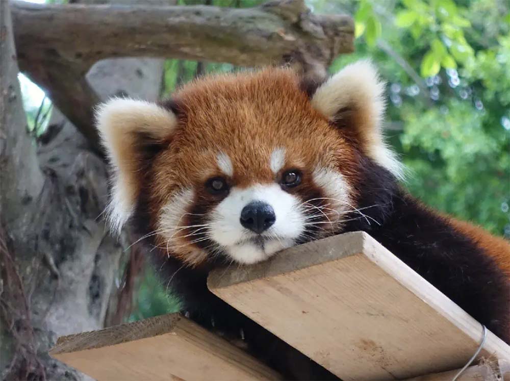
Answer:
The image features a close-up view of a red panda resting on a wooden platform. The panda is characterized by its distinctive red fur, white face, and ears. The background shows a natural setting with green foliage and a wooden structure.
Here are the parameters with descriptions:
python test_ov_internvl2.py --help
usage: Export InternVL2 Model to IR [-h] [-m MODEL_ID] -ov OV_IR_DIR [-d DEVICE] [-pic PICTURE] [-p PROMPT] [-max MAX_NEW_TOKENS] [-llm_int4_com] [-vision_int8] [-llm_int8_quant] [-convert_model_only]
options:
  -h, --help   show this help message and exit
  -m MODEL_ID, --model_id MODEL_ID   model_id or directory for loading
  -ov OV_IR_DIR, --ov_ir_dir OV_IR_DIR     output directory for saving model
  -d DEVICE, --device DEVICE   inference device
  -pic PICTURE, --picture PICTURE  picture file
  -p PROMPT, --prompt PROMPT    prompt
  -max MAX_NEW_TOKENS, --max_new_tokens MAX_NEW_TOKENS    max_new_tokens
  -llm_int4_com, --llm_int4_compress  llm int4 weight scompress
  -vision_int8, --vision_int8_quant  vision int8 weights quantize
  -llm_int8_quant, --llm_int8_quant      llm int8 weights dynamic quantize
  -convert_model_only, --convert_model_only      convert model to ov only, do not do inference test
Supported optimizations
1. Vision model INT8 quantization and SDPA optimization enabled
2. LLM model INT4 compression
3. LLM model INT8 dynamic quantization
4. LLM model with SDPA optimization enabled
Summary
This blog introduces how to use the OpenVINO™ python API to run the pipeline of the Internvl2-4B model, and uses a variety of acceleration methods to improve the inference speed.
moondream2 model enabling with OpenVINO
Introduction
moondream2 is a small vision language model designed to run efficiently on edge devices. Although the model has a small number of parameters, it provides high-performance visual processing capabilities. It can quickly understand and process input images and respond to user queries. The model was developed by VikhyatK and is released under the permissive Apache 2.0 license, allowing for commercial use.
You can find more information on github repository: https://github.com/zhaohb/moondream2-ov
OpenVINOTM backend on moondream2
Step 1: Install system dependency and setup environment
Create and enable python virtual environment
conda create -n ov_py310 python=3.10 -y
conda activate ov_py310
Clone themoondream2-ov repository from gitHub
git clone https://github.com/zhaohb/moondream2-ov
cd moondream2-ov
Install python dependency
pip install -r requirement.txt
pip install --pre -U openvino openvino-tokenizers --extra-index-url https://storage.openvinotoolkit.org/simple/wheels/nightly
Step 2: Get HuggingFace model
git lfs install
git clone https://hf-mirror.com/vikhyatk/moondream2
git checkout 48be9138e0faaec8802519b1b828350e33525d46
Step 3: Export OpenVINO™ models and simple inference test with OpenVINO™
python3 test_ov_moondream2.py -m /path/to/moondream2 -o /path/to/moondream2_ov
Question: Describe this image.
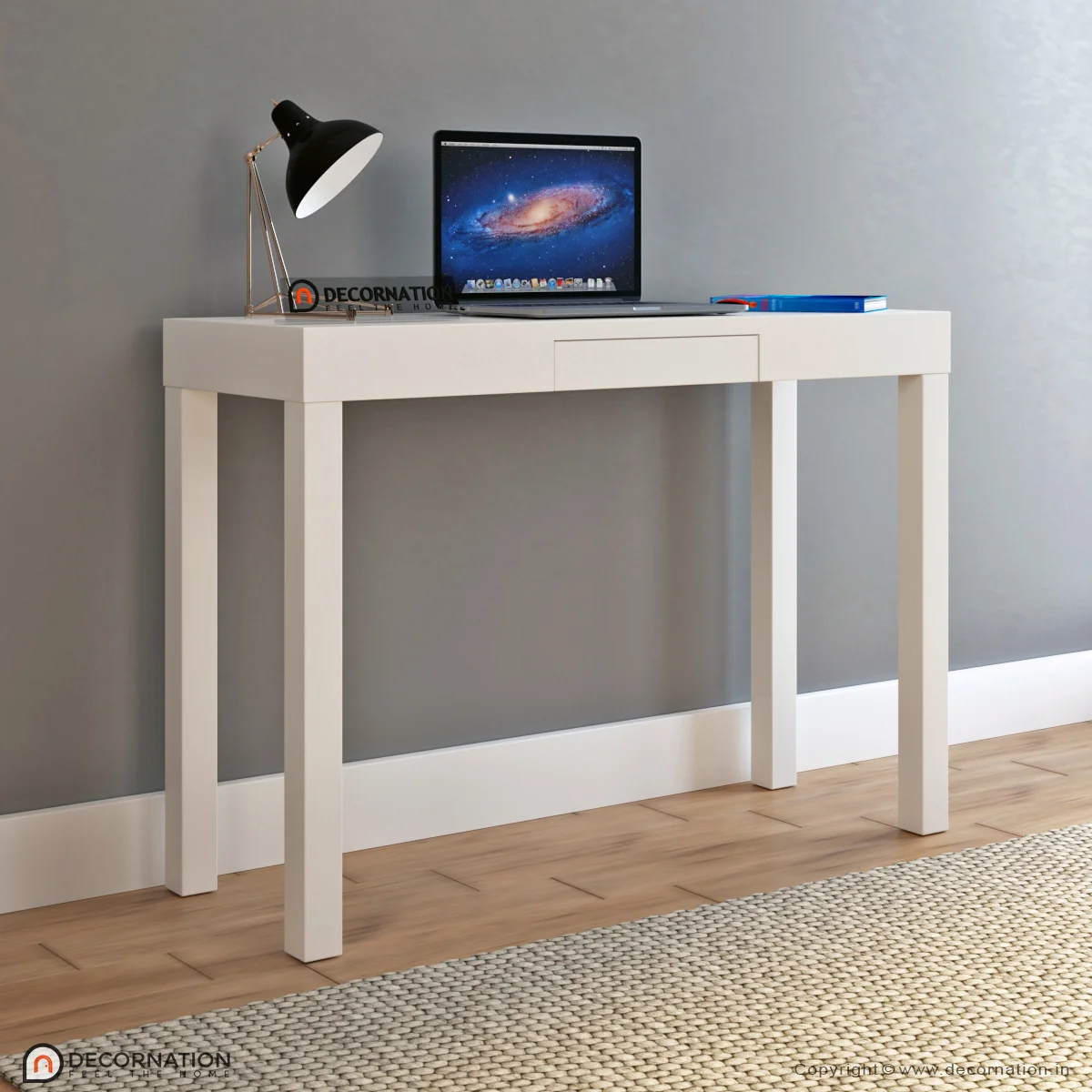
Answer:
The image shows a modern white desk with a laptop, a lamp, and a notebook on it, set against a gray wall and a wooden floor.
Optimizing MeloTTS for AIPC Deployment with OpenVINO: A Lightweight Text-to-Speech Solution
Authors : Qiu Tong, Zhao Hongbo
MeloTTS released by MyShell.ai, is a high-quality, multilingual Text-to-Speech (TTS) library that supports English, Chinese (mixed English), and various other languages. The strengths of the model lie in its lightweight design, which is well-suited for applications on AIPC systems, coupled with its impressive performance. In this article, I will guide you through the process of converting the model to be compatible with OpenVINO toolkits, enabling it to run on various devices such as CPUs, GPUs and NPUs. Additionally, I will provide a concise overview of the model's inference procedure.
Overview of Model Inference Procedure and Pipeline
For each language type, the pipeline requires only two models (two inference procedures). For instance, English language generation necessitates just the 'bert-base-uncased' model and its corresponding MeloTTS-English. Similarly, for Chinese language generation (which includes mixed English), the pipeline needs only the 'bert-base-multilingual-uncased' and MeloTTS-Chinese. This greatly streamlines the pipeline compared to other TTS frameworks, and the compact size of the models makes them suitable for deployment on edge devices.
MeloTTS is based on Variational Inference with adversarial learning for end-to-end Text-to-Speech (VITS). The inference process is illustrated in the figure. It encompasses a text encoder, a stochastic duration predictor, a decoder.
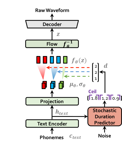
The text encoder accepts phones, tones and a hidden layer from a BERT model as input. It then produces the text encoder's output along with its mean value and a logarithmic variance. To align the input texts with the target speech, the outputs from the encoders are processed using a stochastic duration predictor, which generates an alignment matrix. This matrix is then used to expand the mean value and a logarithmic variance (assuming a Gaussian distribution) to obtain the results for the latent variables .Subsequently, the inverse flow transformation is applied to obtain the distribution of final latent variable z, which represents the spectrogram. In the decoder, by upsampling the spectrogram, the final audio waveform is obtained.
def ov_infer(self, phones=None, phones_length=None, speaker_id=None, tones=None, lang_ids=None, bert=None, ja_bert=None, sdp_ratio=0.2, noise_scale=0.6, noise_scale_w=0.8, speed=1.0):
The inference entry is the function. In practical inference, phone refers to the distinct speech sounds, while tone refers to the vocal pitch contour. For Chinese, a phone corresponds to pinyin, and a tone corresponds to one of the four tones. In English, phones are the consonants and vowels, and tones relate to stress patterns. Here, noise_scale and noise_scale_w do not refer to actual noise. Both noise_scale_w and noise_scale are components within the Stochastic Duration Predictor, used to introduce randomness in order to enhance the expressiveness of the model.
Note that MeloTTS does not include a voice cloning component, unlike the majority of other TTS models, which makes it more lightweight. If voice cloning is required, please refer to OpenVoice.
Enable Model for OpenVINO
As previously mentioned, the pipeline requires just two models for each language. Taking English as an example, we must first convert both 'bert-base-uncased' and 'MeloTTS-English' into the OpenVINO IR format.
        example_input={
                "x": x_tst,
                "x_lengths": x_tst_lengths,
                "sid": speakers,
                "tone": tones,
                "language": lang_ids,
                "bert": bert,
                "ja_bert": ja_bert,
                "noise_scale": noise_scale,
                "length_scale": length_scale,
                "noise_scale_w": noise_scale_w,
                "sdp_ratio": sdp_ratio,
            }

        ov_model = ov.convert_model(
            self.model,
            example_input=example_input,
        )
        get_input_names = lambda: ["phones", "phones_length", "speakers",
                                  "tones", "lang_ids", "bert", "ja_bert",
                                  "noise_scale", "length_scale", "noise_scale_w", "sdp_ratio"]
        for input, input_name in zip(ov_model.inputs, get_input_names()):
            input.get_tensor().set_names({input_name})
        outputs_name = ['audio']
        for output, output_name in zip(ov_model.outputs, outputs_name):
            output.get_tensor().set_names({output_name})
        """
        reshape model
        Set the batch size of all input tensors to 1
        """
        shapes = {}
        for input_layer  in ov_model.inputs:
            shapes[input_layer] = input_layer.partial_shape
            shapes[input_layer][0] = 1
        ov_model.reshape(shapes)

        ov.save_model(ov_model, Path(ov_model_path))
For instance, we convert the MeloTTS-English model from the pytorch format directly by utilizing the openvino.convert_model API along with pseudo input data.
Note that the input and output layers (it is optional) are renamed to facilitate subsequent development. Furthermore, the batch dimension for all inputs is fixed at 1, as multiple batches are not required here (this is also optional).
We further quantized both the BERT and TTS models to int8 using pseudo data. We observed that our method of quantizing the TTS model introduces a slight distortion to the current sound. To suppress this, we implemented DeepFilterNet, which is also very lightweight.
More about model conversion and int8 quantization please refer to MeloTTS-OV .
Run BERT part on NPU
To enhance performance and reduce CPU offloading, we can shift the execution of the BERT model to the NPU on Meteor Lake.
To adapt the model for the NPU, we've converted the model to accept static shape inputs a and pad each input during inference.
def reshape_for_npu(model, bert_static_shape = 32):
        # change dynamic shape to static shape
        shapes = dict()
        for input_layer  in model.inputs:
            shapes[input_layer] = bert_static_shape
        model.reshape(shapes)
        ov.save_model(model, Path(ov_model_save_path))
        print(f"save static model in {Path(ov_model_save_path)}")

def main():
    core = Core()
    model = core.read_model(ov_model_path)
    reshape_for_npu(model, bert_static_shape=bert_static_shape)
Simple Demo
Here are the audio files generated by the int8 quantized model from OpenVINO.
https://github.com/zhaohb/MeloTTS-OV/tree/speech-enhancement-and-npu/demo
Q3'24: Technology Update – Low Precision and Model Optimization
Authors
Alexander Kozlov, Nikita Savelyev, Vui Seng Chua, Souvikk Kundu, Nikolay Lyalyushkin, Andrey Anufriev, Pablo Munoz, Alexander Suslov, Liubov Talamanova, Yury Gorbachev, Nilesh Jain, Maxim Proshin
Summary
This quarter, we continue observing the trendon the optimization of LLM-based pipelines. Besides a high interest in weight quantizationto precisions beyond 4-bits, we see a lot of effort in the optimization of usageof KV-cache during the ScaledDotProduct computation: from KV-cache quantizationand decomposition to sparse attention where only a part of KV-cache is used topredict the next token. This gives the opportunity to design more efficientinference pipelines with heterogeneous execution (see RetrievalAttention work).
Highlights
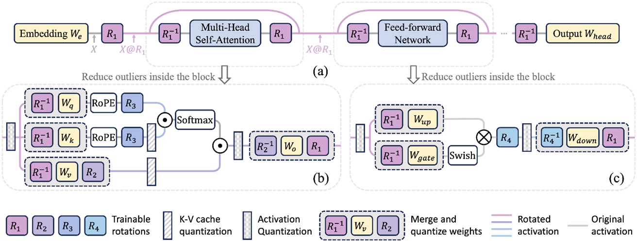
- SpinQuant: LLM Quantizationwith Learned Rotations by Meta (https://arxiv.org/abs/2405.16406). Develop the idea of rotation by a random orthogonal matrix from QuIP, QuIP#, and QuaRotto reduce outliers in the LLMs and obtain better quality of W4A4KV4 quantization. The authors found that not all rotations help equally, and random rotations produce a significant variance in quantized models. Therefore, it is proposed to search for “good” rotation matrices using optimization with Cayley optimization. The matrix optimization procedure takes a little over an hour on smaller representatives of the LLama family on 8 A100 and half a day for 70B models. Regarding quality, they are ahead of baselines (the closest QuaRot is about 1% on average). Adding a rotation inside FFN gives the most significant gain. Code is available: https://github.com/facebookresearch/SpinQuant.
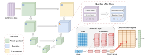
- ACCURATE COMPRESSION OFTEXT-TO-IMAGE DIFFUSION MODELS VIA VECTOR QUANTIZATION by Yandex Research, HSE University, Skoltech, MIPT, Neural Magic, IST Austria (https://arxiv.org/pdf/2409.00492).The authors explore vector-based PTQ strategies for text-to-image diffusion models and demonstrate that the compressed models yield higher quality text-to-image generation than the scalar alternatives under the same bit-widths. They describe an effective fine-tuning technique that further closes the gap between the full-precision and compressed models, leveraging the flexibility of the vector quantized representation. To showcase the method, they compress the weights of SDXL down to 3 bits per parameter. Extensive human evaluation and automated metrics confirm the superiority of our approach over previous diffusion compression methods under the same bit-widths. The authors illustrate that the approach can be effectively applied to distilled diffusion models, such as SDXL, which achieve nearly lossless 4-bit compression. Code is available at https://github.com/yandex-research/vqdm.
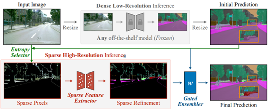
- Sparse Refinement for Efficient High-Resolution Semantic Segmentation by MIT, NVIDIA, Tsinghua University, University of Toronto, UC Berkeley (https://arxiv.org/pdf/2407.19014). Authors introduce a novel approach that enhances dense low-resolution predictions with sparse high-resolution refinements. Based on coarse low-resolution outputs, the method first uses an entropy selector to identify a sparse set of pixels with high entropy. It then employs a sparse feature extractor to generate the refinements for those pixels of interest. Finally, it leverages a gated ensembler to apply these sparse refinements to the initial coarse predictions. The method can be seamlessly integrated into any existing semantic segmentation model, regardless of CNN- or ViT-based. SparseRefine achieves significant speedup: 1.5 to 3.7 times when applied to HRNet-W48, SegFormer-B5, Mask2Former-T/L and SegNeXt-L on Cityscapes, with negligible to no loss of accuracy.
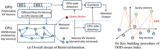
- RetrievalAttention: Accelerating Long-Context LLM Inference via Vector Retrieval by Microsoft Research, Shanghai Jiao Tong University, Fudan University (https://arxiv.org/pdf/2409.10516). Authors employ dynamic sparse attention during token generation, allowing the most critical tokens to emerge from the extensive context data. To address theOOD issue, the method constructs a vector index tailored for the attention mechanism, focusing on the distribution of queries rather than key similarities. This approach allows for traversal of only a small subset of key vectors (1% to 3%), effectively identifying the most relevant tokens to achieve accurate attention scores and results. To optimize resource utilization, RetrievalAttention retains KV vectors in the GPU memory following static patterns while offloading the majority of KV vectors to CPU memory for index construction. This strategy enables RetrievalAttention to perform attention computation with reduced latency and minimal GPU memory utilization. The method shows SOTA results in terms of latency-performance.
Papers with notable results
Quantization
- ADFQ-ViT: Activation-Distribution-Friendly Post-Training Quantization for Vision Transformers by Chinese universities (https://arxiv.org/pdf/2407.02763). Authors design the Per-Patch Outlier-aware Quantizer and the Shift-Log2 Quantizer, which addresses the challenges of outliers and irregular distributions in post-LayerNorm activations and the non-uniform distribution of positive and negative values in post-GELU activations. They also introduce the attention-score enhanced module-wise optimization, which optimizes the parameters of the weight and activation quantizer to reduce errors before and after quantization. The method shows very good results for various Vision Transformer models and use cases at W4A4 and W6A6 setups.
- How Does Quantization Affect Multilingual LLMs? by Cohere (https://arxiv.org/pdf/2407.03211). The authors investigate the problem of LLM accuracy degradation after quantization. They use automatic benchmarks, LLM-as-a-Judge methods, and human evaluation, finding that (1) harmful effects of quantization are apparent in human evaluation, and automatic metrics severely underestimate the detriment: a 1.7%average drop in Japanese across automatic tasks corresponds to a 16.0% drop reported by human evaluators on realistic prompts; (2) languages are disparately affected by quantization, with non-Latin script languages impacted worst; and (3) challenging tasks such as mathematical reasoning degrade fastest.
- CLAMP-ViT: Contrastive Data-Free Learning for Adaptive Post-Training Quantization of ViTs by Georgia Institute of Technology and Intel Labs (https://arxiv.org/pdf/2407.05266). The authors incorporate a patch-level contrastive learning scheme to generate richer, semantically meaningful data. Furthermore, they leverage contrastive learning in layer-wise evolutionary search for fixed- and mixed-precision quantization to identify optimal quantization parameters while mitigating the effects of a non-smooth loss landscape. Evaluations across various vision tasks demonstrate the superiority of CLAMP-ViT, with performance improvements of up to 3% in top-1 accuracy for classification, 0.6 mAP for object detection, and 1.5 mIoU for segmentation at a similar or better compression ratio over existing alternatives. The code is available at https://github.com/georgia-tech-synergy-lab/CLAMP-ViT.git.
- RoLoRA: Fine-tuning Rotated Outlier-free LLMs for Effective Weight-Activation Quantization by Hong Kong University of Science and Technology and Meta Reality Labs (https://arxiv.org/pdf/2407.08044).The paper proposes RoLoRA, the scheme for weight-activation quantization. RoLoRA utilizes rotation for outlier elimination and proposes rotation-aware fine-tuning to preserve the outlier-free characteristics in rotated LLMs. Experimental results show RoLoRA consistently improves low-bit LoRA convergence and post-training quantization robustness in weight-activation settings. The code is supposed to be available at https://github.com/HuangOwen/RoLoRA.
- LRQ: Optimizing Post-Training Quantization for Large Language Models by Learning Low-Rank Weight-Scaling Matrices by NAVER Cloud, KAIST AI, AITRICS, SNU AI Center (https://arxiv.org/pdf/2407.11534). The authors propose a post-training weight quantization method for LLMs that reconstructs the outputs of an intermediate Transformer block by leveraging low-rank weight-scaling matrices, replacing the conventional full weight-scaling matrices that entail as many learnable scales as their associated weights. Thanks to parameter sharing via low-rank structure, the method only needs to learn significantly fewer parameters while enabling the individual scaling of weights, thus boosting the generalization capability of quantized LLMs. Authors show the superiority of the method over prior LLM PTQ works under (i) 8-bit weight and per-tensor activation quantization, (ii) 4-bitweight and 8-bit per-token activation quantization, and (iii) low-bitweight-only quantization schemes. The code is available at https://github.com/onliwad101/FlexRound_LRQ.
- AdaLog: Post-Training Quantization for Vision Transformers with Adaptive Logarithm Quantizer by Beihang University (https://arxiv.org/pdf/2407.12951). The paper proposes a non-uniform quantizer that optimizes the logarithmic base to accommodate the power-law-like distribution of activations while simultaneously allowing for hardware-friendly quantization and dequantization. By employing the bias reparameterization, the quantizer is applicable to both the post-Softmax and post-GELU activations. The authors also develop an efficient Fast Progressive Combining Search (FPCS) strategy to determine the optimal logarithm base, as well as the scaling factors and zero points for the uniform quantizers. Experimental results on public benchmarks demonstrate promising results for various ViT-based architectures and vision tasks, especially in the W6A6setup. The code is available at https://github.com/GoatWu/AdaLog.
- RECLAIMING RESIDUAL KNOWLEDGE: A NOVEL PARADIGM TO LOW-BITQUANTIZATION by Irish Universities (https://arxiv.org/pdf/2408.00923). The authors present an efficient, low-bit, and PTQ framework for ConvNets by framing optimal quantization as an architecture search problem to re-capture quantization residual knowledge with low-rank adapters. They introduce a differentiable neural combinatorial optimization approach, searching for the optimal low-rank adapters using a smooth, high-order normalized Butterworth kernel. They also show a result, converting the weights of existing high-rank quantization residual convolutional operators to low-rank adapters without training. The method achieves good 4-bit and 3-bit quantization results by using less than 250 iterations on a small calibration set with 1600 images. Code will be open-sourced.
- VQ4DiT: Efficient Post-Training Vector Quantization for Diffusion Transformers by Zhejiang University and vivo Mobile Communication (https://arxiv.org/pdf/2408.17131). The authors explore the Vector Quantization methods for extremely low bit-width DiTs and introduce DiT-specific improvements for better quantization. They calibrate both the codebook and the assignments of each layer simultaneously. The proposed method calculates the candidate assignment set for each weight sub-vector based on Euclidean distance and reconstructs the sub-vector based on the weighted average. Then, using the zero-data and block-wise calibration method, the optimal assignment from the set is efficiently selected while calibrating the codebook. The method achieves competitive evaluation results compared to full-precision models on the ImageNet.
- MobileQuant: Mobile-friendly Quantization for On-device Language Models by Samsung AI Center, Cambridge (https://arxiv.org/pdf/2408.13933). The authors introduce a post-training quantization approach for LLMs that is supported by current mobile hardware implementations (i.e., DSP, NPU), thus being directly deployable on real-edge devices. The method improves upon prior works through simple yet effective methodological extensions that enable us to effectively quantize most activations to a lower bit-width (i.e., 8-bit) with near-lossless performance. They conduct an on-device evaluation of model accuracy, inference latency, and energy consumption. The results indicate that the proposed method reduces inference latency and energy usage by 20%-50% while still maintaining accuracy compared to models using 16-bit activations.
- Low-Bit width Floating Point Quantization for Efficient High-Quality Diffusion Models by the University of Toronto & Vector Institute (https://arxiv.org/pdf/2408.06995).The authors propose a floating-point quantization method for diffusion models that provides better image quality compared to integer quantization methods. They employ a floating-point quantization method by integrating weight rounding learning during the mapping of the full-precision values to the quantized values in the quantization process. The authors also study integer and floating-point quantization methods in state-of-the-art diffusion models. Additionally, they introduce a methodology to evaluate quantization effects, highlighting shortcomings with existing output quality metrics and experimental methodologies. Finally, their floating-point quantization method increases model sparsity by an order of magnitude, enabling further optimization opportunities.
- DopQ-ViT: Towards Distribution-Friendly and Outlier-Aware Post-Training Quantization for Vision Transformers by Institute of Automation and School of Artificial Intelligence of Chinese Academy of Sciences (https://arxiv.org/pdf/2408.03291v2).The paper focuses on the full quantization of Vision Transformers. The authors propose using the Tan Quantizer, which focuses more on values near 1, thereby better fitting the distribution of post-Softmax activations in Transformer layers. Besides, the method selects the median as the optimal scaling factor, effectively addressing the accuracy degradation issue that occurs after parametrizing post-LayerNorm activations. The method achieves very accurate results especially in W6/A6 for various tasks such as ImageNet or MS COCO.
- Differentiable Product Quantization for Memory Efficient Camera Relocalization by Czech Technical University in Prague, Aalto University, University of Oulu (https://arxiv.org/pdf/2407.15540).The authors introduce a simple and standalone metric learning for Differentiable Product Quantization for 3D scene compression that preserves matching properties of the descriptors and the final camera localization performance; ii) the proposed hybrid method enables a better tradeoff between memory complexity and localization; iii) they analyze the tradeoffs between description and map compression and show how localization is more tolerant to description compression on outdoor and indoor datasets. The code will be publicly available at https://github.com/AaltoVision/dpqe.
- Advancing Multimodal Large Language Models with Quantization-Aware Scale Learning for Efficient Adaptation by Xiamen University and SkyWork AI (https://arxiv.org/pdf/2408.03735).The paper introduces a Quantization-aware scale Learning method based on multimodal warmup. This method is grounded in two key innovations: (1) The learning of group-wise scale factors for quantized LLM weights to mitigate the quantization error arising from activation outliers and achieve more effective vision-language instruction tuning; (2) The implementation of a multimodal warmup that progressively integrates linguistic and multimodal training samples, thereby preventing overfitting of the quantized model to multimodal data while ensuring stable adaptation of multimodal large language models to downstream vision-language tasks. The code is supposed to be available at https://github.com/xjjxmu/QSLAW.
- Mamba-PTQ: Outlier Channels in Recurrent Large Language Models by Intel Labs (https://arxiv.org/pdf/2407.12397).This workshop paper is among the first to study post-training quantization on the Mamba architecture. Similar to Transformer models, it observed the presence of outlier channels in activations (those with absolute maximum values exceeding 6 standard deviations from the layer mean) and found that downstream task performance degrades substantially when these channels are removed. The study presents zero-shot results of naïve symmetrical per-tensor quantization of weights and activations across Mamba1 models, ranging from 130M to 2.8B parameters, providing a baseline for future quantization research on this emerging architecture.
- Foundation of Large Language Model Compression – Part 1: Weight Quantization by CSAIL MIT (https://arxiv.org/pdf/2409.02026).This work introduces CVXQ, a post-training weight quantization framework that assigns varying bit widths down to the per-group level, constrained by a target average bit rate per weight element. Formulated through the lens of Lagrangian convex optimization, the framework leads to a dual-ascent methods that alternately update the bit width and the tradeoff variable until all optimality conditions are met. To overcome the non-differentiability arising from discrete bit widths and considering that weight distributions are Gaussian or Laplacian, the framework leverages a well-known result from rate-distortion theory to provide closed-form derivative estimates during optimization. CVXQ adopts an interesting compounding (non-uniform) quantization, where weights are first projected to the sigmoid domain before applying uniform round-to-nearest quantization. A codebook is employed to enable dequantization via simple lookup, avoiding complex inverse computations. Tested across a wide range of model sizes in OPT and Llama2, CVXQ outperforms GPTQ, AWQ, and OWQ at 3- and 4-bit rates per weight in nearly all cases. Full implementation will be available soon here.
Pruning / Sparsity
- LazyLLM: DYNAMIC TOKEN PRUNING FOR EFFICIENT LONGCONTEXT LLM INFERENCE by Apple and Meta AI (https://arxiv.org/pdf/2407.14057). The paper introduces an LLM acceleration method that selectively computes the KV for tokens important for the next token prediction in both the prefilling and decoding stages. Contrary to static pruning approaches that prune the prompt at once, LazyLLM allows language models to dynamically select different subsets of tokens from the context in different generation steps, even though they might be pruned in previous steps. The method also introduces a concept of AuxCache to store the tokens that are omitted during the previous steps of text generation but required at the current step. Experiments on standard datasets across various tasks demonstrate that LazyLLM can significantly accelerate the generation without fine-tuning, e.g., prefilling stage of the LLama 2 7B model by 2.34x while maintaining accuracy.
- Compact Language Models via Pruning and Knowledge Distillation by Nvidia (https://www.arxiv.org/pdf/2407.14679). Authors propose compression best practices for LLMs that combine depth, width, attention, and MLP pruning with knowledge distillation-based retraining. They arrive at these best practices through a detailed empirical exploration of pruning strategies for each axis, methods to combine axes, distillation strategies, and search techniques for arriving at optimal compressed architectures. They use this guide to compress the Nemotron-4 family of LLMs by a factor of 2-4× and compare their performance to similarly-sized models on a variety of language modeling tasks. Deriving 8B and 4B models from an already pretrained 15B model using this approach requires up to 40x fewer training tokens per model compared to training from scratch; this results in compute cost savings of 1.8x for training the full model family (15B, 8B, and 4B).
- SQFT: Low-cost Model Adaptation in Low-precision Sparse Foundation Models by Intel Labs (https://github.com/IntelLabs/Hardware-Aware-Automated-Machine-Learning). This paper proposes an end-to-end solution for low-precision sparse parameter-efficient fine-tuning of large pre-trained models. It includes an innovative strategy that enables the merging of sparse weights with low-rank adapters without losing the sparsity induced in the base model, overcoming the limitations of previous approaches. SQFT also addresses the challenge of having quantized weights and adapters with different numerical precisions, enabling merging in the desired numerical format without sacrificing accuracy. Multiple adaptation scenarios, models, and comprehensive sparsity levels demonstrate the effectiveness of SQFT. Models and open-source code are available.
- ShadowLLM: Predictor-based Contextual Sparsity for Large Language Models by Cornell University and Google (https://arxiv.org/abs/2406.16635). Contemporary research on contextual sparsity primarily uses magnitude-based metrics to measure the importance of attention heads and neurons in LLMs. This paper aims to assess various importance metrics from the literature, including those based on(1) activation norm, (2) first-order gradient, (3) combination of norm and gradient, (4) second-order gradient, and (5) sensitivity-based metrics. The authors conclude that the PlainAct criterion – the L1-norm of the product of magnitude and gradient – emerges as the better metric by offering a robust sparsity-task tradeoff and learnability in importance rank. The authors also propose using just a single predictor, with the attention scores of the first transformer block as input, to forecast sparsity patterns for the entire LLM, as opposed to DejaVu, which requires predictors at regular intervals of transformer blocks. This innovation simplifies predictor training and implementation while also reducing inference overhead, achieving up to 20% faster generation than DejaVu across sizes of OPT family. Code is here.
- STUN: Structured-Then-Unstructured Pruning for Scalable MoE Pruning by SNU and Snowflake AI Research (https://arxiv.org/pdf/2409.06211). The work discovers a novel way to prune experts of MoE where the method reduces the complexity of expert selection from combinatorial O(kn/√n) down to O(1) using several greedy assumptions. The authors exploit the structure of router weight, applying clustering based on a so-called behavioral similarity metric to identify (dis)similar experts and utilize the centroid as pruned representation to compute a first-order Taylor approximation of the relative distortion. The entire expert pruning can be effectively run without any calibration data and unnecessarily on GPU, especially for the MoE with large numbers of experts. The work also found that expert pruning followed by unstructured pruning provides a better Pareto front. A key result on Snowflake Arctic, a 480B-parameter MoE with 128 experts, shows that STUN achieves 40% sparsity with minimal performance loss in just two hours using a single H100 GPU where unstructured pruning methods alone fall short.
Other
- Accuracy is Not All You Need by Microsoft Research, India (https://arxiv.org/pdf/2407.09141). The authors study the accuracy difference between compressed and source models. They claim that when the accuracy metrics are similar, they observe the phenomenon of flips, wherein answers change from correct to incorrect and vice versa in proportion. The authors conduct a detailed study of metrics across multiple compression techniques, models, and datasets, demonstrating that the behavior of compressed models as visible to end users is often significantly different from the baseline model, even when accuracy is similar. They further evaluate compressed models qualitatively and quantitatively using MT-Bench, showing that compressed models are significantly worse than baseline models in this free-form generative task. They argue that compression techniques should also be evaluated using distance metrics. Finally, the authors propose two metrics, KL-Divergence and % flips, and show that they are well correlated.
- Scaling LLM Test-Time Compute Optimally can be More Effective than Scaling Model Parameters by UC Berkeley and Google DeepMind (https://arxiv.org/pdf/2408.03314).The paper studies the scaling of inference-time computation in LLMs, focusing on answering the question: If an LLM is allowed to use a fixed but non-trivial amount of inference-time compute, how much can it improve its performance on a challenging prompt? Answering this question has implications not only on the achievable performance of LLMs, but also on the future of LLM pretraining and how one should trade inference-time and pre-training compute. Authors analyze two primary mechanisms to scale test-time computation: (1) searching against dense, process-based verifier reward models; and (2) updating the model’s distribution over a response adaptively, given the prompt at test time. They find that in both cases, the effectiveness of different approaches to scaling test-time compute critically varies depending on the difficulty of the prompt. This observation motivates applying a “compute-optimal” scaling strategy, which acts to most effectively allocate test-time compute adaptively per prompt. Using this compute-optimal strategy, authors can improve the efficiency of test-time compute scaling by more than 4x compared to a best-of-N baseline. Additionally, in a FLOPs-matched evaluation, they find that on problems where a smaller base model attains somewhat non-trivial success rates, test-time compute can be used to outperform a 14x larger model.
- Transformers are SSMs: Generalized Models and Efficient Algorithms Through Structured State Space Dual it by Tri Dao and Albert Gu (https://arxiv.org/abs/2405.21060). This paper discusses improvements to Mamba, the selective structure state space model (SSM) proposed as an alternative to Transformer-based models. The authors provide a framework called State Space Duality (SSD) that connects SSMs and variants of the attention mechanism. The Mamba-2 architecture is proposed, which obtains 2-8x speedup compared to the previous version of Mamba, and it is designed to be friendly to tensor and sequence parallelism. Experiments show that Mamba-2 outperforms Mamba and Transformer-based models in different model sizes. The authors also discuss hybrid models that can benefit from the combination of SSD with components from Transformer blocks.
Software
- A thorough analysis of performance and bottlenecks when using 4-bit KV cache on Nvidia with PyTorch: https://pytorch.org/blog/int4-decoding. Authors show step-by-step improvement when computing the Self-Attention operation of the Transformer block and compare results with CUDA and Flash Decoding baselines in 4-bit per-row and per-channel quantization settings of KV-cache.
- Llama.cpp introduced SIMD-friendly ternary weights packing/unpacking: https://compilade.net/blog/ternary-packing
- HuggingFace posted an exploratory work and recipes for ternary weights (1.58 bits) LLM weight compression: https://huggingface.co/blog/1_58_llm_extreme_quantization.
Enable 2D Lip Sync Wav2Lip Pipeline with OpenVINO Runtime
Authors: Xiake Sun, Kunda Xu
1. Introduction
Lip sync technologies are widely used for digital human use cases, which enhance the user experience in dialog scenarios.
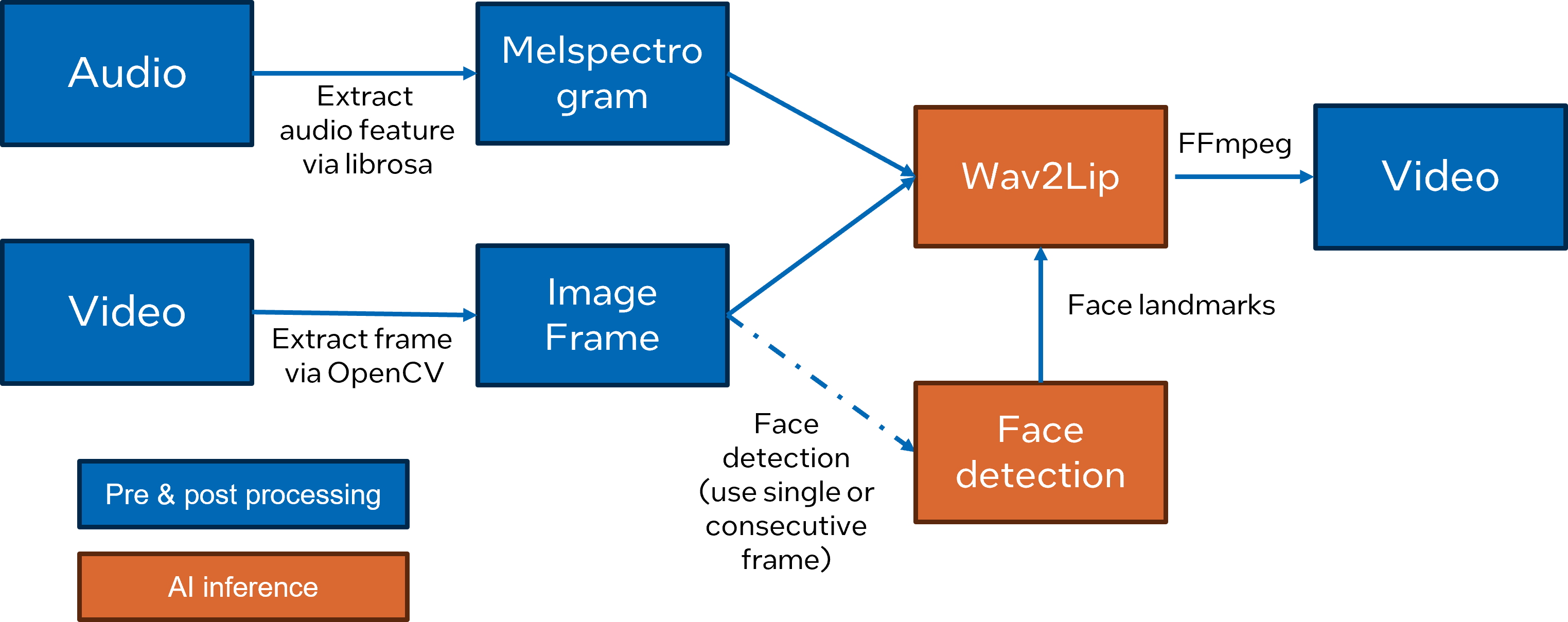
Wav2Lip is a novel approach to generate accurate 2D lip-synced videos in the wild with only one video and an audio clip. Wav2Lip leverages an accurate lip-sync “expert" model and consecutive face frames for accurate, natural lip motion generation.
In this blog, we introduce how to enable and optimize Wav2Lippipeline with OpenVINOTM.
Here is Wav2Lip pipeline overview:
2. Setup Environment
Download the Wav2lip pytorch model from link and move it to the checkpoints folder.
3. Pytorch to OpenVINOTM Model Conversion
The exported OpenVINOTM model will be saved in the checkpoints folder.
4. Run pipeline inference with OpenVINOTM Runtime
Here are the parameters with descriptions:
--face_detection_path: path of face detection OpenVINOTMIR
--wav2lip_path: path of wav2lip openvinoTM IR
--inference_device: specify the device to run OpenVINOTMinference.
--face: input video with face information
--audio: input audio with voice information
--static: set True to use single frame for face detection for fast inference
The generated video will be saved as results/result_voice.mp4
Here is an example to compare original video and generated video after the Wav2Lip pipeline:
.gif)

5. Conclusion
In this blog, we introduce how to deploy wav2lip pipeline with OpenVINOTM as follows:
- Support Pytorch model to OpenVINOTM model conversion.
- Run and optimize wav2lip pipeline with OpenVINOTM runtime.
OpenVINO Enable Digital Human-TTS (GPT-SoVITs)
Authors : Kunda, Xu / Aidova, Ekaterina
Introduction
GPT-SoVITS is a powerful voice cloning model that supports a small amount of voice conversion and text-to-speech. It supports voice reasoning in Chinese, English, and Japanese.
You only need to provide a 5-second voice sample to experience voice cloning with 80%~95% similarity. If you provide a 1-minute voice sample, you can get close to the effect of a real person and train a high-quality TTS model!
As the founder of RVC Voice Changer (GitHub nickname: RVC-Boss), he recently opened up a cross-language voice cloning project. GPT-SoVITs has attracted highly praised recommendations from the industry as soon as it went online, and it has received 1.4k Stars on GitHub in less than two days. Its voice cloning effect close to that of a real person and the use of Zero-short have made GPT-SoVITs highly recognized in the field of digital humans.
Although there are many tutorials on how to use GPT-SoVITs online, in this article I will show you how to optimize it through OpenVINO and deploy it on the CPU. GPT-SoVITs belongs to the category of TTS tasks, but the difference is that it can add sound features to the generated audio by introducing additional reference audio (ref_wav), making the output audio effect closer to real people speaking.
The pipeline structure of GPT-SoVITs
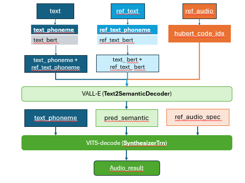
GPT-SOVITS adds a residual quantization layer to the original SOVITS input. Referring to VALL-E, the input of this quantization layer contains the text features and timbre features of the audio. GPT-SoVITs mainly consists of four parts: text preprocessing, audio preprocessing, VALL-E, VITS-decode
- Text preprocessing :
Convert text encoding information (text_ids) into pronunciation encoding information (phoneme_ids)
Use the Bert model to encode the phoneme_ids information, and take the third-to-last layer tensor as the result output
Phoneme features and Bert features are phoneme features for text, similar to pinyin
- Audio preprocessing :
Use the cn_hubert_encoder model to sample the audio information and extract the code_ids of ref_audio
Based on ref_audio, extract the frequency ref_audio_spec frame feature
- VALL-E:
Use for predict pred_sementic and idx, The idx is used to truncate pred_sementic (remove the features of the reference audio)
- VITs-decode :
Use VITS-decode to decode and get the output
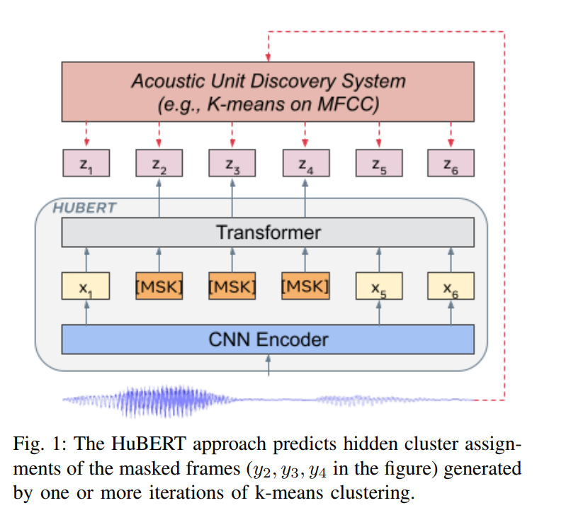
HuBert sub model
The HuBert model is designed to extract audio autoencoder features and is developed by the Facebook AI research team. The goal is to learn a universal speech representation that can capture important information in speech signals, such as speech content, speaker identity, emotional state, etc. These representations can be used in a variety of downstream tasks, such as automatic speech recognition (ASR), speaker identification, sentiment analysis, etc.
Reference paper : https://arxiv.org/pdf/2106.07447
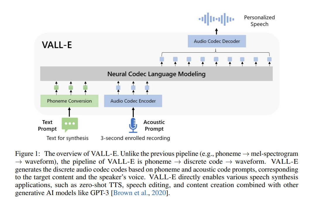
VALL-E sub model
VALL-E is a neural codec model developed by Microsoft Research, focusing on the field of speech synthesis. The characteristic of VALL-E is that it can generate synthesized speech that meets the speech characteristics of the target speaker through a small number of target speech samples (such as a 3-second speech clip). VALL-E completes the generation of speech coding based on Encoder. The GPT module of GPT-SOVITS implements the process from text to speech coding. Referring to SOVITS, a residual quantization layer is added to the original entrance. The input of this quantization layer contains the text features and timbre features of the audio.
Reference paper : https://arxiv.org/pdf/2301.02111
SoVITs sub model
The core module of GPT-SOVITS is not much different from SOVITS, which is an end-to-end text-to-speech(TTS) synthesis model. It combines variational inference and adversarial learning to generate high-quality, natural-sounding speech. It is still divided into two parts:
- Generator based on VAE + FLOW
- Discriminator based on multi-scale classifier
Reference paper : https://arxiv.org/pdf/2106.06103
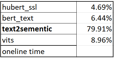
By counting the inference time of the entire GPT-SoVITs pipeline, we found that the two models with the largest time overhead are text2sementic (VALL-E) and vits (VITs-decode). The total overhead of the two models accounts for 87% of the entire pipeline. Therefore, optimizing these two models through OpenVINO is very necessary to improve the performance of the entire pipeline.
You canrefer to the sample code snippet to achieve this. OpenVINO enables HuBert, Bert, VALL-E, VITs 4 sub models, and builds the pipeline based on OpenVINO.
Reference GitHub project : 18582088138/GPT-SoVITS-OpenVINO:[OpenVINO Enable]1 min voice data can also be used to train a good TTS model! (few shot voice cloning) (github.com)
Export HuBert model code snippet
HuBert sub model definition
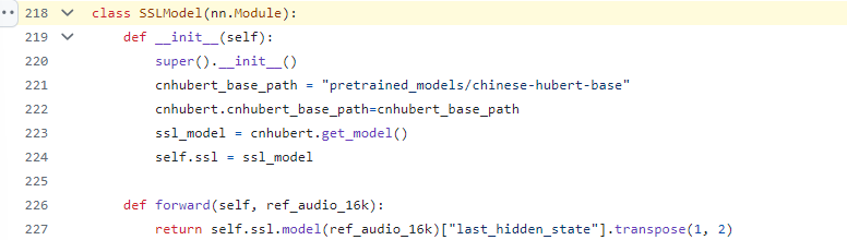
HuBert sub model convert

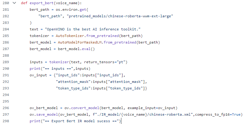
Export Bert model code snippet
Bert sub model definition and convert
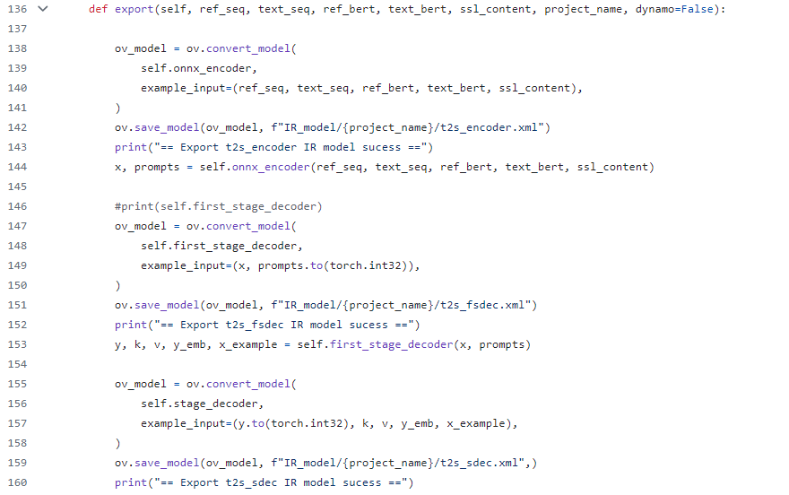
Export VALL-E model code snippet
Since t2sis defined as three modules in the source code: t2s_encoder, first_stage_decoder, stage_decoder, refer to its source code implementation and convert these three modules into corresponding IR models through OpenVINO.
However, if the generated class model can refer to the Transformer basic model for KV cache optimization, the performance of the t2s model will be further improved, but this requires some code development work, and I will add this function in subsequent work (To Do).
VALL-E sub model definition
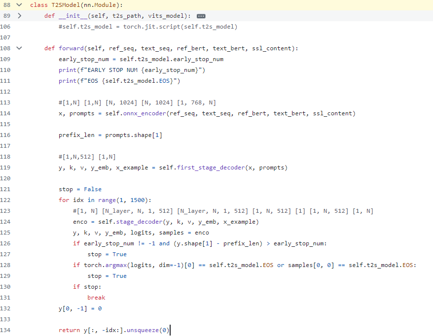
VALL-E sub model convert
Export VITs sub model code snippet
In the VITs model, the spectrogram torch function has two operators "torch.hann_window" and "torch.stft". Currently, OpenVINO opset does not support these two operators. Therefore, this part temporarily needs to use the operators in torch opset and redefine the original VITs sub-model. After the subsequent operators are successfully supported, OpenVINO will re-enable the VITs model (To Do).
VITs sub model definition
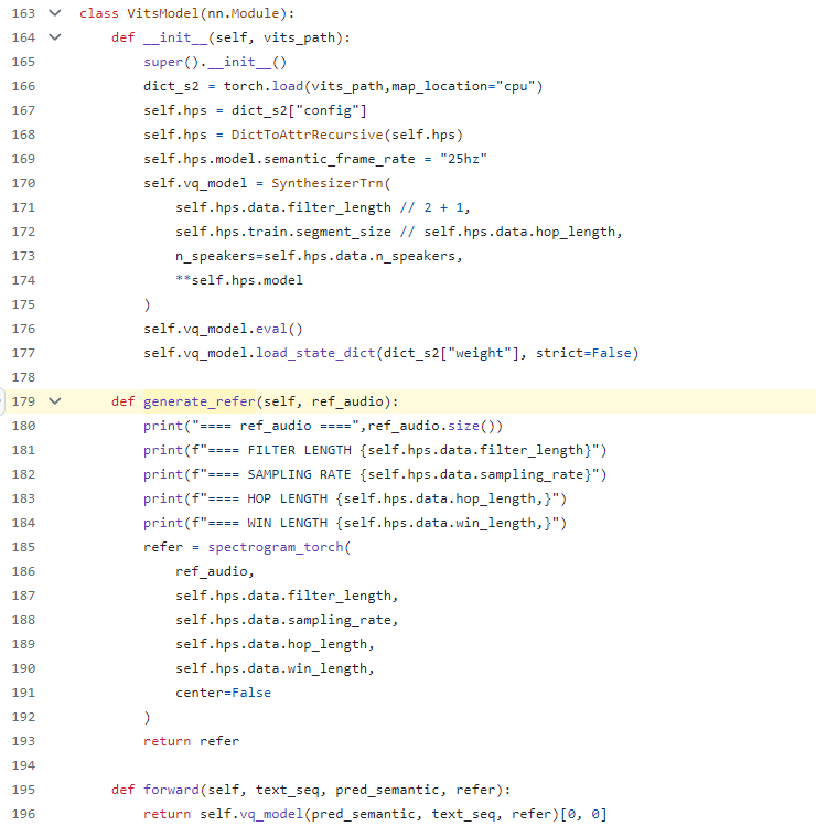
VITs sub model convert
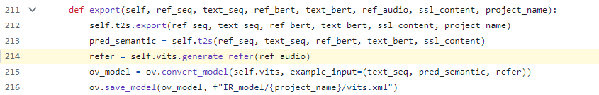
Finally, we rebuilt the GPT-SoVITs pipeline through the four sub models enabled by OpenVINO. You can refer to the implementation of the pipeline:
Reference link : GPT-SoVITS-OpenVINO/GPT_SoVITS/ov_pipeline_gpt_sovit.py at 18582088138/GPT-SoVITS-OpenVINO(github.com)