

OpenVINO Blog

Enable LoRA weights with Stable Diffusion Controlnet Pipeline
Authors: Zhen Zhao(Fiona), Kunda Xu
Low-Rank Adaptation(LoRA) is a novel technique introduced to deal with the problem of fine-tuning Diffusers and Large Language Models (LLMs). In the case of Stable Diffusion fine-tuning, LoRA can be applied to the cross-attention layers for the image representations with the latent described. You can refer HuggingFace diffusers to understand the basic concept and method for model fine-tuning: https://huggingface.co/docs/diffusers/training/lora
In this blog, we aimed to introduce the method building up the pipeline for Stable Diffusion + ControlNet with OpenVINO™ optimization, and enable LoRA weights for Unet model of Stable Diffusion to generate images with different styles. The demo source code is based on: https://github.com/FionaZZ92/OpenVINO_sample/tree/master/SD_controlnet
Stable Diffusion ControlNet Pipeline
Step 1: Environment preparation
First, please follow below method to prepare your development environment, you can choose download model from HuggingFace for better runtime experience. In this case, we choose controlNet for canny image task.
* Please note, the diffusers start to use `torch.nn.functional.scaled_dot_product_attention` if your installed torch version is >= 2.0, and the ONNX does not support op conversion for “Aten:: scaled_dot_product_attention”. To avoid the error during the model conversion by “torch.onnx.export”, please make sure you are using torch==1.13.1.
Step 2: Model Conversion
The demo provides two programs, to convert model to OpenVINO™ IR, you should use “get_model.py”. Please check the options of this script by:
In this case, let us choose multiple batch size to generate multiple images. The common application of vison generation has two concepts of batch:
- `batch_size`: Specify the length of input prompt or negative prompt. This method is used for generating N images with N prompts.
- `num_images_per_prompt`: Specify the number of images that each prompt generates. This method is used to generate M images with 1 prompts.
Thus, for common user application, you can well use these two attributes in diffusers to generate N*M images by N prompts with increased random seed values. For example, if your basic seed is 42, to generate N(2)*M(2) images, the actual generation is like below:
- N=1, M=1: prompt_list[0], seed=42
- N=1, M=2: prompt_list[0], seed=43
- N=2, M=1: prompt_list[1], seed=42
- N=2, M=2: prompt_list[1], seed=43
In this case, let’s use N=2, M=1 as a quick example for demonstration, thus the use`--batch 2`. This script will generate static shape model by default. If you are using different value of N and M, please specify `--dynamic`.
Please check your current path, make sure you already generated below models currently. Other ONNX files can be deleted for saving space.
- controlnet-canny.<xml|bin>
- text_encoder.<xml|bin>
- unet_controlnet.<xml|bin>
- vae_decoder.<xml|bin>
* If your local path already exists ONNX or IR model, the script will jump tore-generate ONNX/IR. If you updated the pytorch model or want to generate model with different shape, please remember to delete existed ONNX and IR models.
Step 3: Runtime pipeline test
The provided demo program `run_pipe.py` is manually build-up the pipeline for StableDiffusionControlNet which refers to the original source of `diffusers.StableDiffusionControlNetPipeline`
The difference is we simplify the pipeline with 4 models’ inference by OpenVINO™ runtime API which can make sure the model inference can be accelerated on Intel® CPU and GPU platform.
The default iteration is 20, image shape is 512*512, seed is 42, and the input image and prompt is for “Girl with Pearl Earring”. You can adjust or custom your own pipeline attributes for testing.
In the case with batch_size=2, the generated image is like below:
Enable LoRA weights for Stable Diffusion
Normal LoRA weights has two types, one is ` pytorch_lora_weights.bin`,the other is using safetensors. In this case, we introduce both methods for these two LoRA weights.
The main idea for LoRA weights enabling, is to append weights onto the original Unet model of Stable Diffusion, then export IR model of Unet which remains LoRA weights.
There are various LoRA models on https://civitai.com/tag/lora , we choose some public models on HuggingFace as an example, you can consider toreplace with your owns.
Step 4-1: Enable LoRA by pytorch_lora_weights.bin
This step introduces the method to add lora weights to Unet model of Stable Diffusion by `pipe.unet.load_attn_procs(...)` function. By using this way, the LoRA weights will be loaded into the attention layers of Unet model of Stable Diffusion.
* Remember to delete exist Unet model to generate the new IR with LoRA weights.
Then, run pipeline inference program to check results.
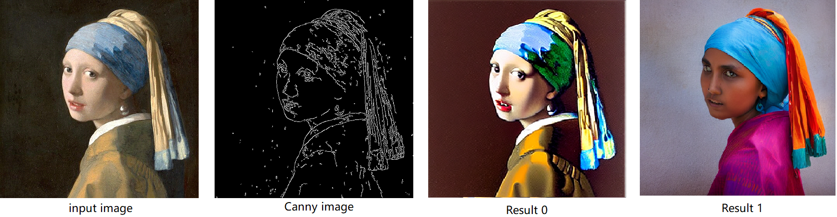
The LoRA weights appended Stable Diffusion model with controlNet pipeline can generate image like below:
Step 4-2: Enable LoRA by safetensors typed weights
This step introduces the method to add LoRA weights to Stable diffusion Unet model by `diffusers/scripts/convert_lora_safetensor_to_diffusers.py`. Diffusers provide the script to generate new Stable Diffusion model by enabling safetensors typed LoRA model. By this method, you will need to replace the weight path to new generated Stable Diffusion model with LoRA. You can adjust value of `alpha` option to change the merging ratio in `W = W0 + alpha * deltaW` for attention layers.
Then, run pipeline inference program to check results.
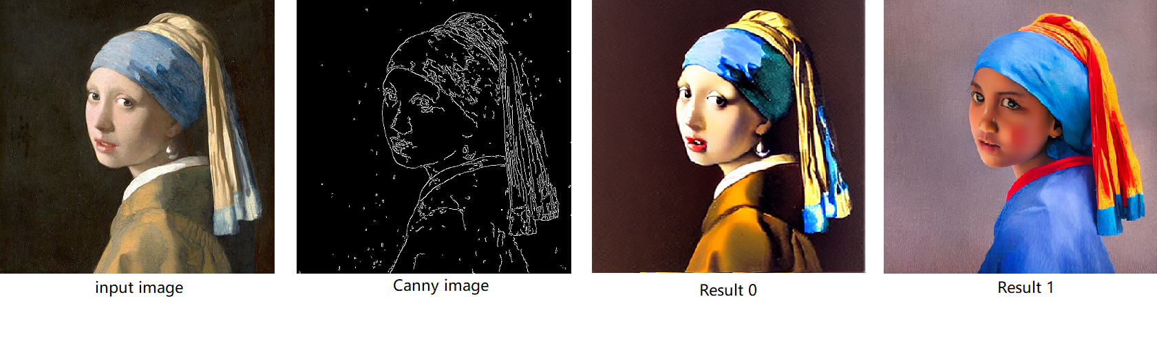
The LoRA weights appended SD model with controlnet pipeline can generate image like below:
Step 4-3: Enable runtime LoRA merging by MatcherPass
This step introduces the method to add lora weights in runtime before Unet or text_encoder model compiling. It will be helpful to client application usage with multiple different LoRA weights to change the image style by reusing the same Unet/text_encoder structure.
This method is to extract lora weights in safetensors file and find the corresponding weights in Unet model and insert lora weights bias. The common method to add lora weights is like:
W = W0 + W_bias(alpha * torch.mm(lora_up, lora_down))
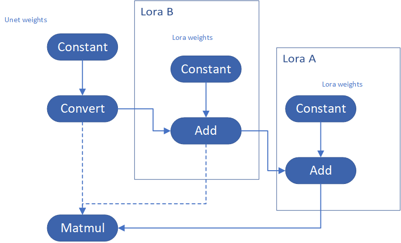
I intend to insert Add operation for Unet's attentions' weights by OpenVINO™ `opset10.add(W0,W_bias)`. The original attention weights in Unet model is loaded by `Const` op, the common processing path is `Const->Convert->Matmul->...`, if we add the lora weights, we should insert the calculated lora weight bias as `Const->Convert->Add->Matmul->...`. In this function, we adopt `openvino.runtime.passes.MatcherPass` to insert `opset10.add()` with call_back() function iteratively.
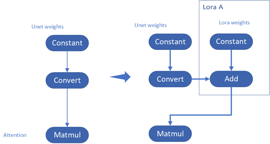
Your own transformation operations will insert opset.Add() firstly, then during the model compiling with device. The graph will do constant folding to combine the Add operation with following MatMul operation to optimize the model runtime inference. Thus, this is an effective method to merge LoRA weights onto original model.
You can check with the implementation source code, and find out the definition of the MatcherPass function called `InsertLoRA(MatcherPass)`:
The `InsertLoRA(MatcherPass)` function will be registered by `manager.register_pass(InsertLoRA(lora_dict_list))`, and invoked by `manager.run_passes(ov_unet)`. After this runtime MatcherPass operation, the graph compile with device plugin and ready for inference.
Run pipeline inference program to check the results. The result is same as Step 4-2.
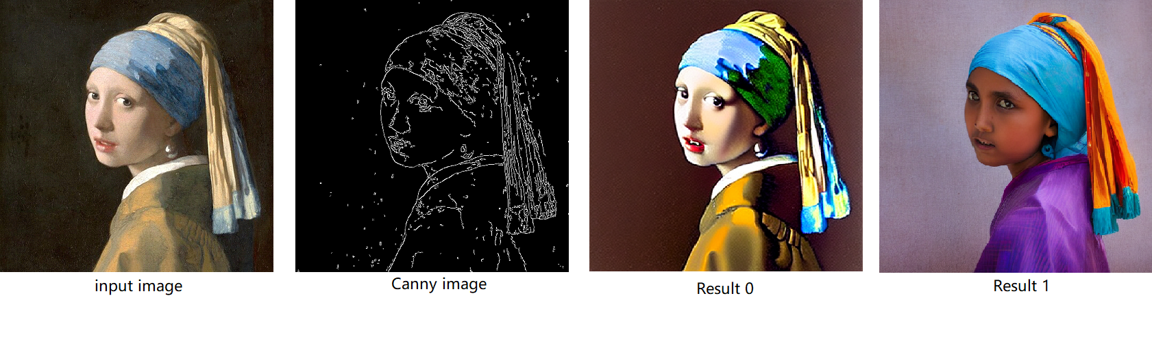
The LoRA weights appended Stable Diffusion model with controlNet pipeline can generate image like below:
Step 4-4: Enable multiple LoRA weights
There are many different methods to add multiple LoRA weights. I list two methods here. Assume you have two LoRA weigths, LoRA A and LoRA B. You can simply follow the Step 4-3 to loop the MatcherPass function to insert between original Unet Convert layer and Add layer of LoRA A. It's easy to implement. However, it is not good at performance.
Please consider about the Logic of MatcherPass function. This fucntion required to filter out all layer with the Convert type, then through the condition judgement if each Convert layer connected by weights Constant has been fine-tuned and updated in LoRA weights file. The main costs of LoRA enabling is costed by InsertLoRA() function, thus the main idea is to just invoke InsertLoRA() function once, but append multiple LoRA files' weights.
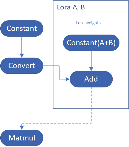
By above method to add multiple LoRA, the cost of appending 2 or more LoRA weights almost same as adding 1 LoRA weigths.
Now, let's change the Stable Diffusion with dreamlike-anime-1.0 to generate image with styles of animation. I pick two LoRA weights for SD 1.5 from https://civitai.com/tag/lora.
- soulcard: https://civitai.com/models/67927?modelVersionId=72591
- epi_noiseoffset: https://civitai.com/models/13941/epinoiseoffset
You probably need to do prompt engineering work to generate a useful prompt like below:
- prompt: "1girl, cute, beautiful face, portrait, cloudy mountain, outdoors, trees, rock, river, (soul card:1.2), highly intricate details, realistic light, trending on cgsociety,neon details, ultra realistic details, global illumination, shadows, octane render, 8k, ultra sharp"
- Negative prompt: "3d, cartoon, lowres, bad anatomy, bad hands, text, error"
- Seed: 0
- num_steps: 30
- canny low_threshold: 100
You can get a wonderful image which generate an animated girl with soulcard typical border like below:

Additional Resources
Provide Feedback & Report Issues
Notices & Disclaimers
Intel technologies may require enabled hardware, software, or service activation.
No product or component can be absolutely secure.
Your costs and results may vary.
Intel does not control or audit third-party data. You should consult other sources to evaluate accuracy.
Intel disclaims all express and implied warranties, including without limitation, the implied warranties of merchantability, fitness for a particular purpose, and non-infringement, as well as any warranty arising from course of performance, course of dealing, or usage in trade.
No license (express or implied, by estoppel or otherwise) to any intellectual property rights is granted by this document.
© Intel Corporation. Intel, the Intel logo, and other Intel marks are trademarks of Intel Corporation or its subsidiaries. Other names and brands may be claimed as the property of others.
Accelerate DIEN for Click-Through-Rate Prediction with OpenVINO™
Author: Xiake Sun, Cecilia Peng
Introduction
A click-through rate (CTR) prediction model is designed to estimate how likely a user will click on an advertisement or item. Deployment of a CTR model is considered one of the core tasks in e-commerce, as its performance not only affects platform revenue but also influences customers’ online shopping experience.
Deep Interest Evolution Network (DIEN) developed by Alibaba Group aims to better predict customer’s CTR to improve the effectiveness of advertisement display. DIEN proposes the following two modules:
- Temporally captures and extracts latent interests based on customer history behaviors.
- Models an evolving process of user interests using GRU with an attentional update gate (AUGRU)
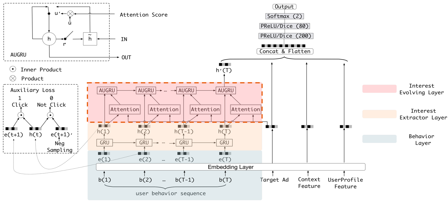
Figure 1 shows the structure of DIEN, with the help of AUGRU, DIEN can overcome the disturbance from interest drifting, which improves the performance of CTR prediction largely in online advertising system.
DIEN Optimization with OpenVINOTM
Here we introduce DIEN optimization with OpenVINOTM in two aspects: graph level and dynamism runtime optimization.
Graph Level Optimization
Figure 2 shows the AUGRU subgraph of DIEN visualized in Netron.
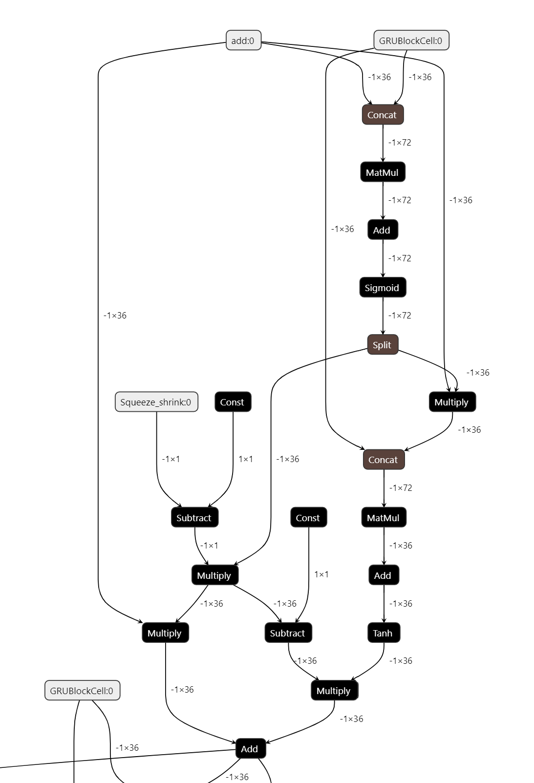
OpenVINOTM implements internal operations AUGRUCell and AUGRUSequence for better graph-level optimization. Each decomposed subgraph of GRU and AUGRU is fused into a corresponding cell operator respectively. What's more, in case of static sequence length, the group of consecutive cells are further fused into a sequence operator. In case of dynamic sequence length, however, the sequence is processed with a loop of cells due to the limitation of oneDNN RNN primitive. This loop of cells is TensorIterator and (AU)GRUCell. We will introduce the optimizations of TensorIterator in next session.
TensorIterator Runtime Optimization with Dynamic Shape
Before we dive into optimization details, let’s first checkout how OpenVINOTM TensorIterator operation works.
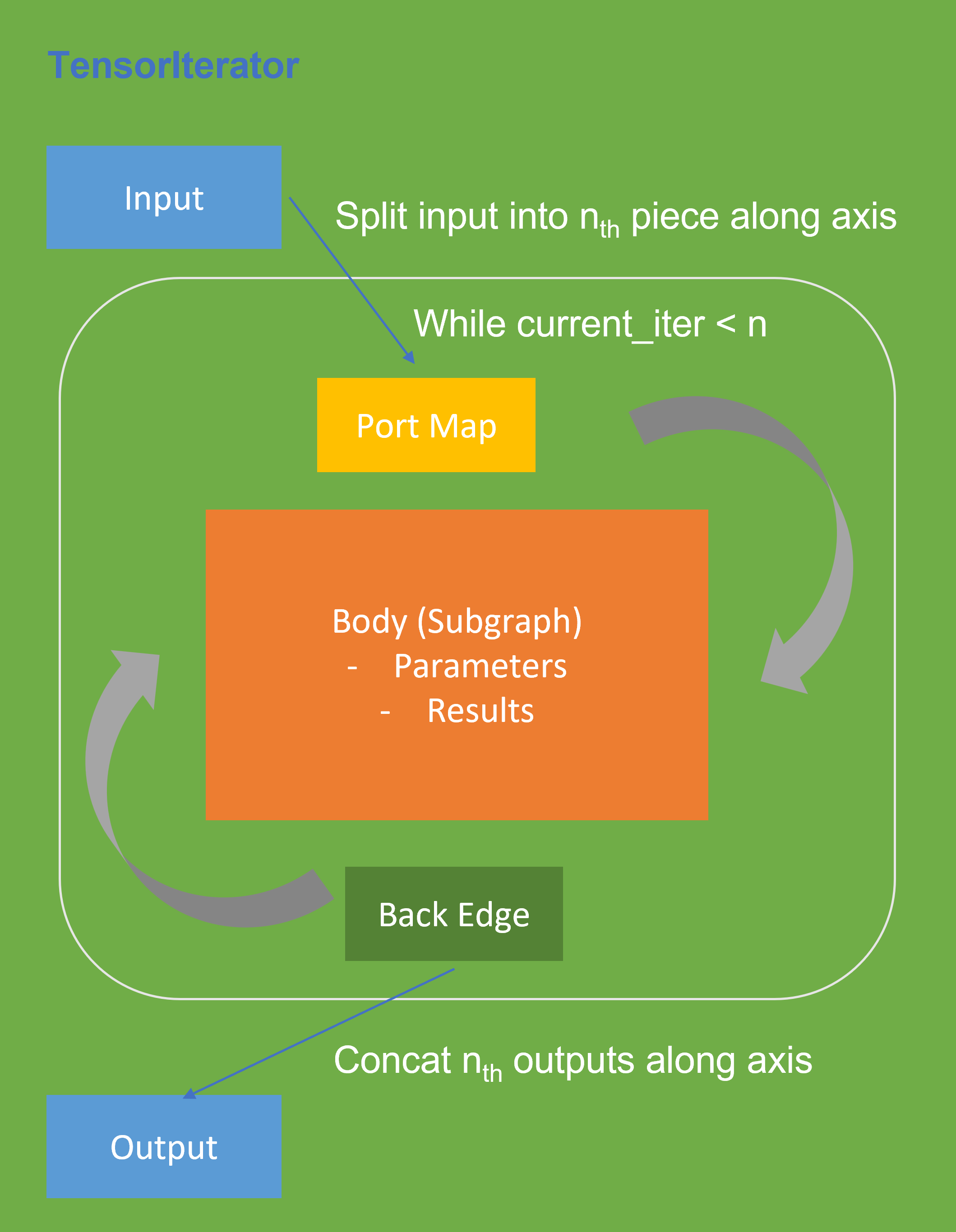
The TensorIterator layer performs recurrent execution of thenetwork, which is described in the body, iterating through the data. Figure 3 shows the workflow of OpenVINOTM Operation TensorIterator in a simplified view. For details, please refer to the specification.
Similar to other layers, TensorIterator has regular sections: input and output. It allows connecting TensorIterator to the rest of the IR. TensorIterator also has several special sections: body, port_map, back_edges. The principles of their work are described below.
- body is a network that will be recurrently executed. The network is described layer by layer as a typical IR network.
- port_map is a set of rules to map input or output data tensors of TensorIterator layer onto body data tensors. The port_map entries can be input and output. Each entry describes a corresponding mapping rule.
- back_edges is a set of rules to transfer tensor values from body outputs at one iteration to body parameters at the next iteration. Back edge connects some Result layers in body to Parameter layer in the same body.
If output entry in the Port map doesn’t have partitioning (axis, begin, end, strides) attributes, then the final value of output of TensorIterator is the value of Result node from the last iteration. Otherwise, the final value of output of TensorIterator is a concatenation of tensors in the Result node for all body iterations.
We use Intel® VTune™ Profiler to run benchmark_app with DIEN FP32 IR model on Intel® Xeon® Gold 6252N Processor for performance profiling.
Cache internal reorder primitives in TensorIterator
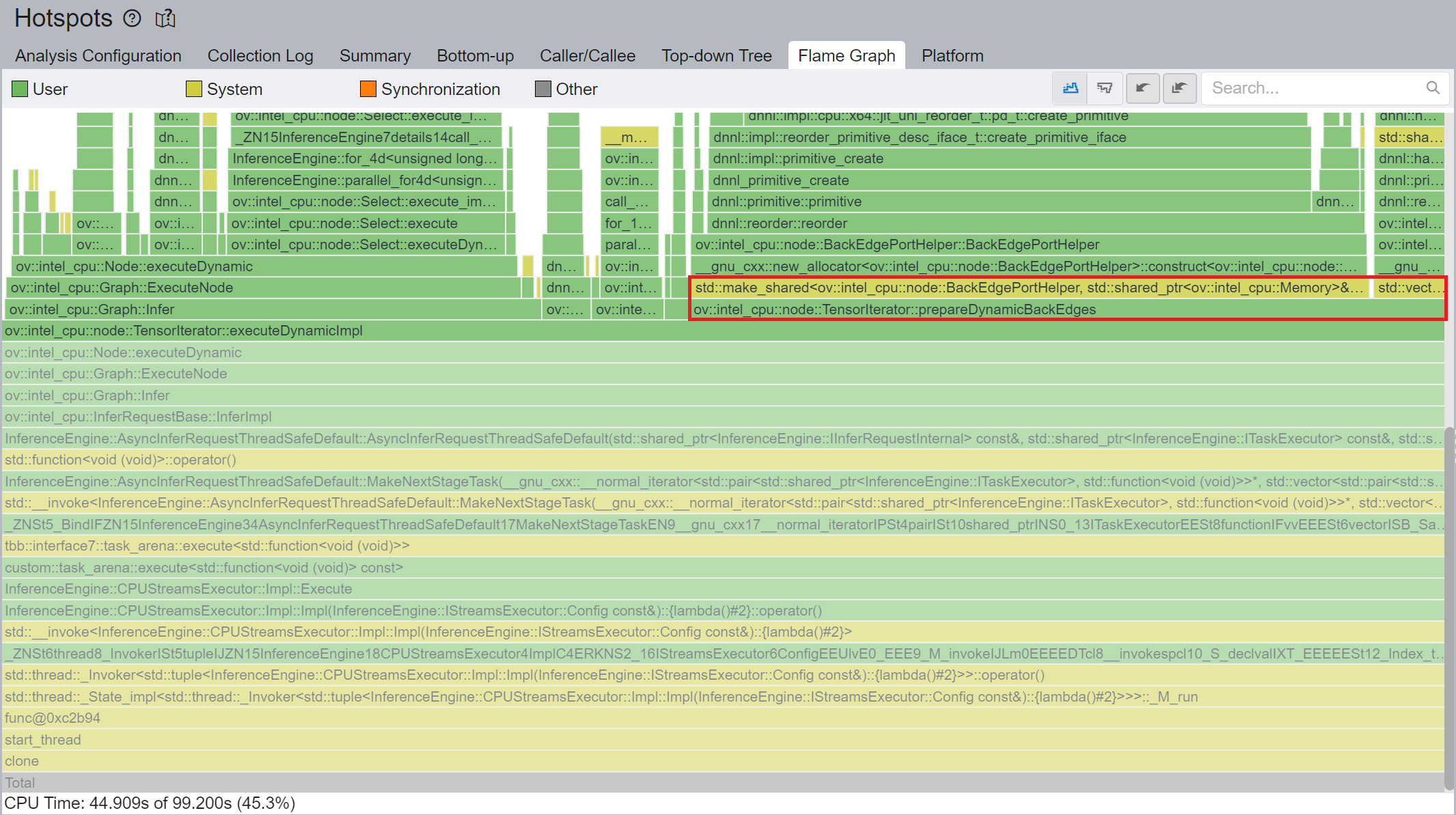
Figure 4 shows that TensorIterator::prepareDynamicBackEdges() spends nearly 45% CPU time to create the reorder primitives. DIEN FP32 model has 2 TensorIterator, eachTensorIterator runs 100 iterations in body with the same input/output shape regarding the current batch. Besides, each TensorIterator has 7 back edges, which means the reorder primitive are frequently created.
So, we propose to cache internal reorder primitive in TensorIterator to optimize back edge memory copy logic. With this optimization, the performance with dynamic shape can be improved by 8x times.
Memory allocation and reuse optimization in TensorIterator
As Figure 3 shows, if we have split input as nth piece to loop in body, at the end, the outputs of TensorIterator will be a concatenation of tensors in the Result node for all body iterations, which can lead to performance overhead. Based on previous optimization we re-run performance profiling using benchmark_app with DIEN FP32 IR model on Intel® Xeon® Gold 6252N Processor as showed in Figure 5.
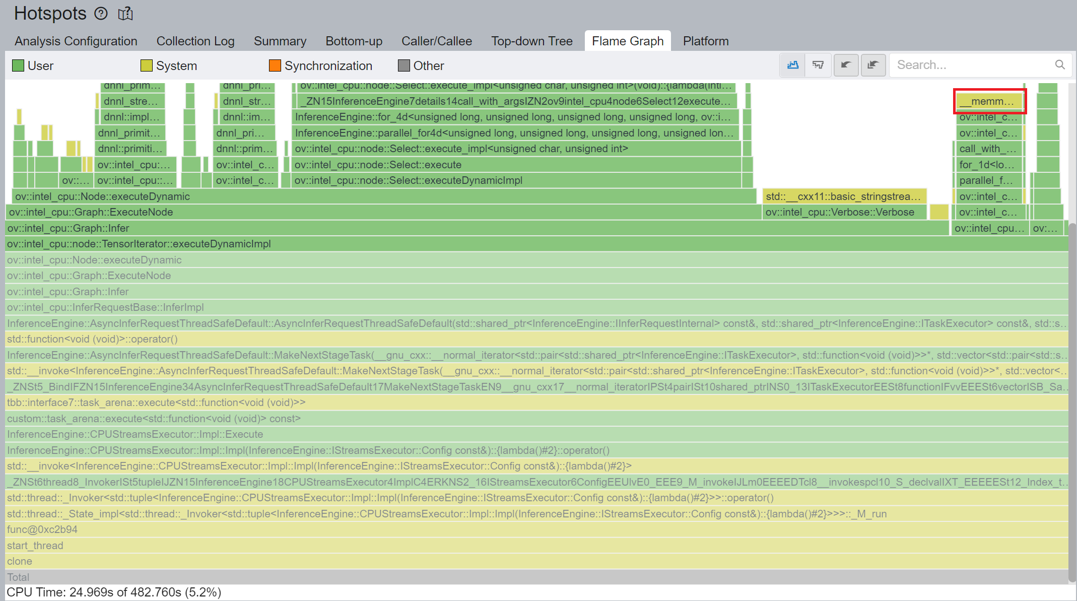
CPU plugin TensorIterator supports both two operators - TensorIterator and Loop. The outputs of each iteration could be concatenated and return to users. Since the output size is not always known before the execution, the legacy implementation is to dynamically allocate the concatenated output buffer.
We propose two points from the memory allocation standpoint:
- In the case of TensorIterator number of iterations is determined by the size of the axis we are slicing. So, if TensorIterator body one ach iteration will produce the same shape on output we can easily preallocate enough memory before the TI computation, The same for Loop with trip count input - we can just read the value from this input, make shape inference for the body and this determines the required amount of memory.
- More complicated story is when we don't know exact number of iterations before Loop inference (e.g., number of iterations is determined by ExecutionCondition input). In that case do the following: let’s have an output buffer where we put the Loop output. Once the buffer doesn't have enough space, we reallocate it on new size based on a simple and effective dynamic array algorithm.
OpenVINOTM implemented memory allocation and reuse optimization in TensorIterator to significantly reduce the number of reallocations and not to allocate to much memory at the same time. Experiments show that performance can be further improved by more than 20%.
DIEN OpenVINOTM Demo
Clone demo repository:
Prepare Amazon dataset:
Setup Python Environment:
Convert original TensorFlow model to OpenVINOTM FP32 IR:
Run the Benchmark with TensorFlow backend:
Run the Benchmark with OpenVINOTM backend using FP32 inference precision:
Run the Benchmark with OpenVINOTM backend using BF16 inference precision:
Please note, Xeon native supports BF16 infer precision since 4th Generation Intel® Xeon® Scalable Processors. Running BF16 on a legacy Xeon platform may lead to performance degradation.
Conclusion
In this blog, we introduce inference optimization of DIEN recommendation model with OpenVINOTM runtime as follows:
- For static input sequence length, AUGRU subgraph will be decomposed and fused as AUGRU and AUGRUSequence OpenVINOTM internal operation.
- For dynamic input sequence length, we propose cache internal reorder primitives and memory allocation and re-use optimization in TensorIterator.
- Provide a demo for model enabling and efficient inference of DIEN with OpenVINOTM runtime.
Reference
Deep Interest Evolution Network (DIEN)
Encrypt Your Dataset and Train Your Model with It Directly
Encrypt Your Dataset and Train Your Model with It Directly

Introduction
When we deal with dataset for creating AI models, we need to consider sensitive information managed and stored online in the cloud or on connected devices. Unsecured datasets can be vulnerable to unauthorized access, theft, and misuse, particularly when processed for machine learning workloads. Certain fields, such as industrial or medical sectors, face exceptionally high risks when their data is exposed to these potential threats. For example, if a dataset used to train a detection model for identifying factory process errors is leaked, it can expose sensitive factory process technology. This highlights the importance of safeguarding datasets at every stage, from data storage to model training.
Dataset Management Framework (Datumaro) offers a dataset encryption feature for AI model training. With Datumaro, you can encrypt datasets of any computer vision data format into the DatumaroBinary format. This encrypted dataset can remain encrypted as far as it is needed for decryption. By combining the encrypted dataset with OpenVINO training extensions™, you can use it directly for model training without decryption. Whenever needed, you can use Datumaro once again to decrypt the dataset and convert it back to any major computer vision data format, such as VOC, COCO, or YOLO. Please refer to another posting data_convert for data convert.
Encrypt Your Dataset Using Datumaro
Datumaro provides two ways to encrypt a dataset: CLI and Python API. First, you need to install Datumaro on your system. Please refer to the installation guide here for detailed instructions. Once you have completed the installation of Datumaro, let's first look at the CLI usage. You can encrypt a dataset using the datum convert CLI command as follows:
The necessary user inputs for this command are as follows:
- -i <input-dataset-path>: Enter the path to the dataset you want to encrypt in <input-dataset-path>.
- -o <output-dataset-path>: Enter the path where the encrypted dataset will be produced in <output-dataset-path>.
NOTE:: (Optional) You can additionally specify the data format of your input dataset by entering the -if <input-dataset-format> argument. In most cases, Datumaro can automatically infer the data format of the input dataset, but it might fail. In such cases, you can use the datum detect --show-rejections <input-dataset-path> command to identify the cause of the failure while inferring the data format.
NOTE:: The --save-media argument is a flag that allows you to convert your media files (e.g., images) as well. If this argument is not provided, the encrypted media will not be included in the output directory and only the encrypted annotations are included in the output directory.
Next, let's take a look at how to encrypt a dataset using the Python API. Please examine the following code snippet:
You import the dataset by specifying the path of the input dataset in the import_from function as path="<input-dataset-path>". Then, to export the dataset, you specify the path of the output dataset in the save_dir="<output-dataset-path>" of the export function. Similarly, you also need to provide the encryption=True and format="datumaro_binary" keyword arguments as in the CLI example. A more detailed end-to-end example for this can be found in a Jupyter notebook. Please refer to this link for more information.
So far, all the examples have used the datumaro_binary (DatumaroBinary) format for the exported dataset. Currently, the dataset encryption feature is only supported for the datumaro_binary format. DatumaroBinary is a Datumaro's own data format that stores annotation data in binary representation. It is much faster and storage efficient compared to string-based datasets such as COCO based on JSON. For more detailed information about DatumaroBinary, please refer to this link.
How Datumaro Encrypts Your Dataset?
Datumaro uses the Fernet symmetric encryption recipe provided by the cryptography library to encrypt the dataset. Fernet is built on top of a number of standard cryptographic primitives such as AES or HMAC, and hence Fernet guarantees that a message encrypted cannot be manipulated or read without the key. Please refer to this link for detailed information.
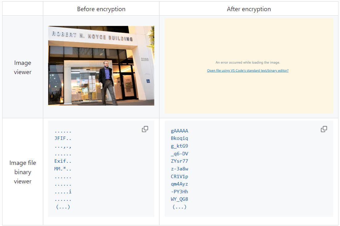
When encrypting the dataset, Datumaro generates a secret key through Fernet and saves it as a txt file at the following path: <output-dataset-path>/secret_key.txt. The secret key generated at this path is a 50-characters string, which consists of a randomly generated 32-bytes string encoded in base64, with the prefix datum- added.
If you have checked the secret key in this file, you must ensure that it is not in the same location with the dataset. If this secret key is uncovered, an attacker would be able to access the contents of the encrypted dataset. Additionally, this secret key is required when training models using OpenVINO training extensions™ with the encrypted dataset or when decrypting it later. Therefore, you should be careful not to lose this secret key.
The following table briefly shows how the data is encrypted. The binary representation of the data is encrypted, so that the following image cannot be seen by the image viewer.
Train Your Model with the Encrypted Dataset Using OpenVINO Training Extensions™
OpenVINO training extensions™ is a tool that allows convenient training of computer vision models and accelerated inference on Intel® devices by exporting trained models to OpenVINO Intermediate Representation (IR) through a CLI. Within the OpenVINO ecosystem, Datumaro is integrated with OpenVINO training extensions™ as a dataset interface. Therefore, the encrypted dataset can be directly used for model training through OpenVINO training extensions™. For detailed installation instructions of OpenVINO training extensions™, please refer to the following link.
Next, let's explore how to use the encrypted dataset directly for model training through the CLI command.
The user inputs required for this command are as follows:
- --train-data-roots <encrypted-dataset-path> and --val-data-roots <encrypted-dataset-path>: Specify the path to the encrypted dataset by replacing <encrypted-dataset-path>. Since the DatumaroBinary format uses the same root directory for both the training and validation subsets, both arguments should have the same value.
- --encryption-key <secret-key>: Provide the secret key corresponding to the encrypted dataset in <secret-key>. This is the 50-character string with the datum- prefix described in the previous section.
NOTE:: <template> is the name of the model template provided by OpenVINO training extensions™. A model template is a recipe for a deep learning model for a specific computer vision task. To explore all the model templates supported by OpenVINO training extensions™, you can use the otx find CLI command or refer to this link.
Decrypt the Encrypted Dataset Using Datumaro
If you want to utilize the encrypted dataset in another AI workload, you need to decrypt the encrypted data. This process reverses the dataset encryption using Datumaro, and encryption-decryption preserves all the information without loss. Similar to the previous section, decryption can be done using the CLI or Python API. Let's first look at decryption using the CLI.
You can use the same datum convert command as before. However, specify the path to the encrypted dataset as the input dataset path (-i <encrypted-dataset-path>), and provide the secret key, which is a 50-character string with the datum- prefix described in the previous section, as the <secret-key> argument for --encryption-key <secret-key>. Additionally, you can choose any data format supported by Datumaro as the output data format. To learn more about the data formats supported by Datumaro, refer to this link.
Next, let's see how decryption can be done using Python API.
Similar to the CLI method, provide the path to the encrypted dataset and the secret key as arguments to the import_from function. For the export function, specify the output dataset path and the output data format.
Conclusion
This post introduced dataset encryption feature provided by Datumaro. It demonstrated how to encrypt a dataset using Datumaro and train a model with the encrypted dataset using OpenVINO training extensions™. Whenever needed you can decrypt it with Datumaro for other AI projects and training frameworks. You can refer to the end-to-end Jupyter notebook example provided on this blog post here for step-by-step guide. The features introduced in this post are available in Datumaro version 1.4.0 or higher and OpenVINO training extensions™ version 1.4.0 or higher.
Datumaro offers a range of useful features for managing datasets besides the dataset encryption feature. You can find examples of other Datumaro features, such as noisy label detection during training with OpenVINO training extensions™, in the Jupyter examples directory. For more information about Datumaro and its capabilities, you can visit the Datumaro documentation page. If you have any questions or requests about using Datumaro, feel free to open an issue here.
Efficient Inference and Quantization of CGD for Image Retrieval with OpenVINO™ and NNCF
Author:Xiake Sun, Wenyi Zou, Churkin Andrey
Introduction
With the advent of e-commerce and online websites, image retrieval applications have been increasing all along around our daily life. Top e-commerce platform such as Amazon and Alibaba have been heavily utilizing image retrieval to put forward what they think is the most suitable product based on what we have seen just now.
Image retrieval is the process of finding an image from a collection or database from the traits of a query image. The traits are usually visual similarities between the images. The top retrieved images can provide hypotheses about which parts of the scene are likely visible in the query image.
Since images in their original form don’t reflect these traits in their pixel-based data, we need to transform this pixel data into a latent space where the representation of the image will reflect the traits. Naver Corporation proposed Combination of Multiple Global Descriptors (CGD) for Image Retrieval task. The CGD framework exploits multiple global descriptors to get an ensemble effect when it can be trained in an end-to-end manner. Quantitative and qualitative analysis results show that exploiting multiple global descriptors led to higher performance over the single global descriptor.
Neural Network CompressionFramework (NNCF) provides a suite of post-training and training-time algorithms for neural network inference optimization in OpenVINO™ with minimal accuracy drop. NNCF is designed to work with models from PyTorch, TensorFlow, ONNX, and OpenVINO™. In this blog, we use NNCF Post-Training Quantization (PTQ) to quantize CGD model, which can further boost inference while keeping acceptable accuracy without fine-tuning.
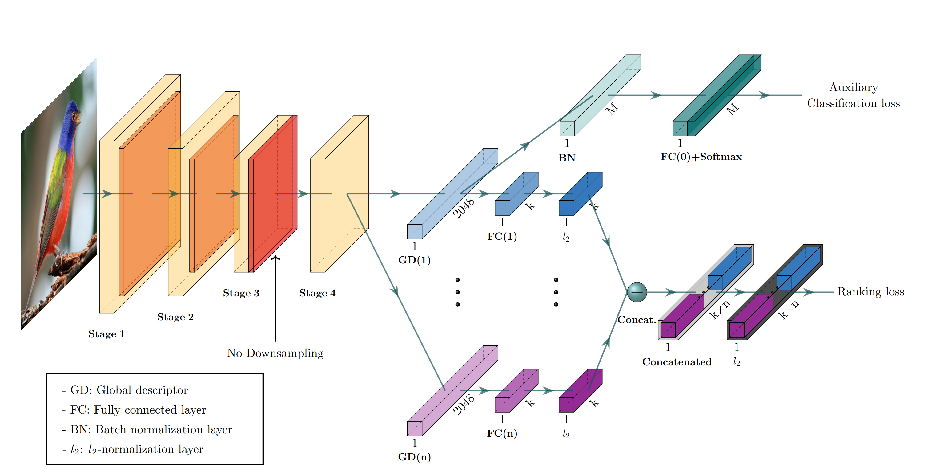
Figure1. shows the CGD framework. The framework is described with ResNet-50 backbone where Stage 3 down sampling is removed. From the last feature map, each of n global descriptor branches outputs a k-dimensional embedding vector, which is concatenated into the combined descriptor for ranking loss. Exclusively the first global descriptor is used for auxiliary classification loss where M denotes the number of classes.
CGD framework utilizes the following global descriptors with different focuses:
- Sum pooling of convolutions (SPoC): activates larger regions on the image representation.
- Generalized mean pooling (GeM): generalizes max and average pooling with a pooling parameter.
- Maximum activation of convolutions (MAC): activates more focused regions.
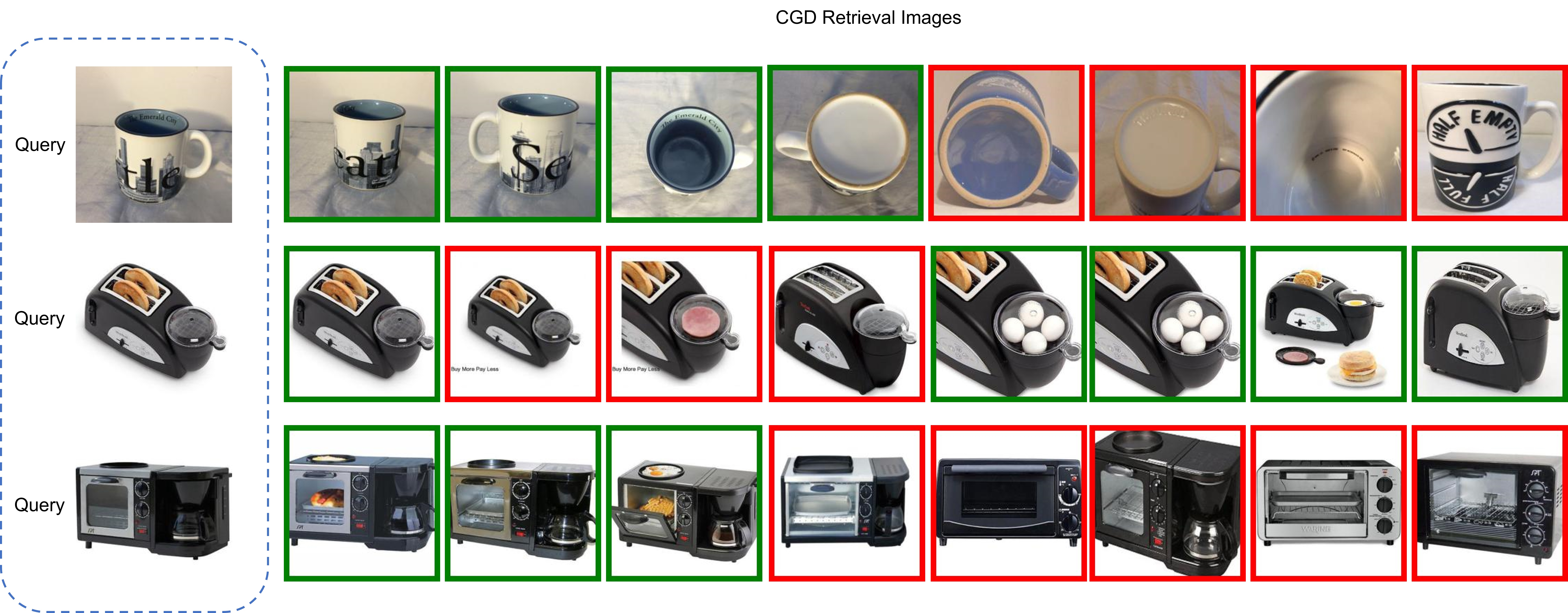
In this blog, we choose CGD ResNet50(SG) model with ResNet50 backbone that combines SPoC and GeM type of global descriptors. Figure 2 shows some retrieval results of CGD Pytorch model based on Standard Online Products (SOP) dataset. The left most query image serves as input to retrieve the 8 most similar image from the database, where the green bounding box means that the predicted class match the query image class, while the red bounding box means a mismatch of image class. Therefore, the retrieved image can be further filtered out with class information.
CGD Model Enabling and Quantization with OpenVINO™ and NNCF
To leverage efficient inference with OpenVINO™ runtime on the intel platform, we proposed the following workflow in Figure 3 for CGD model enabling and quantization with OpenVINO™ and NNCF PTQ, which is implemented in a single Python script run_quantize.py.
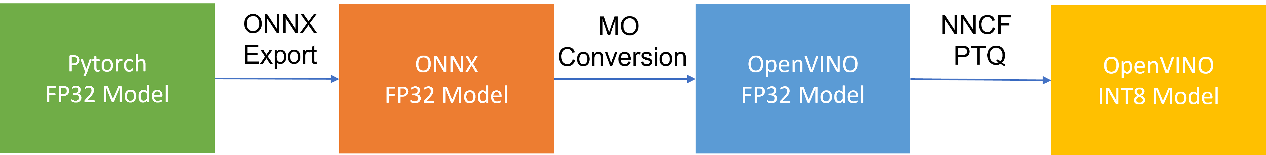
CGD model uses ResNet50 backbone extracted latent feature to create multiple global descriptors, then the global descriptors will be normalized and concatenated as output.
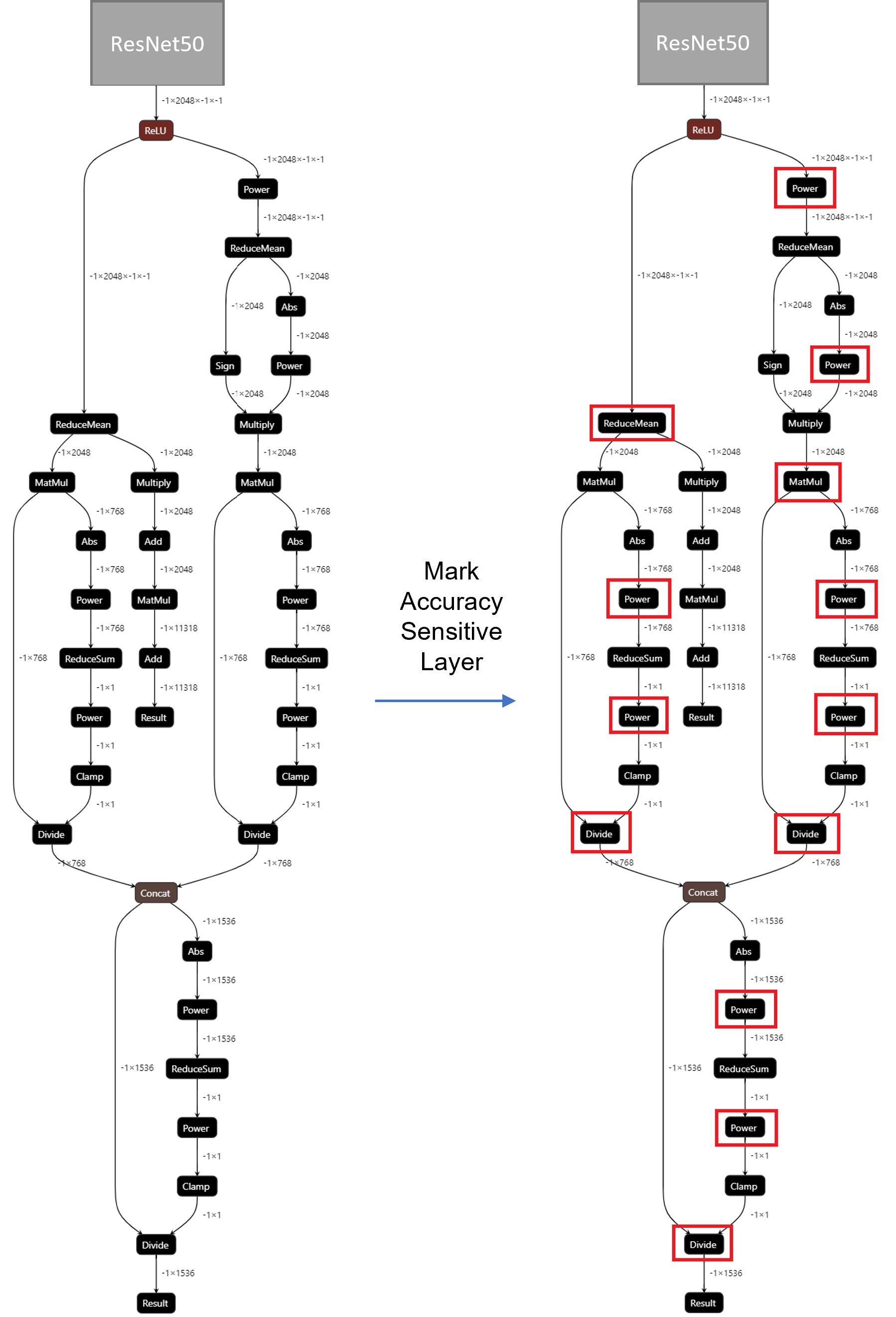
For INT8 quantization, we found some useful tricks to mitigate accuracy issue caused by accuracy sensitive layers, e.g., YOLOv8 OpenVINO Notebook proposes to keep several accuracy sensitive layers in post-processing subgraph as FP32 precision to better preserve accuracy after NNCF PTQ.
For INT8 quantization of CGD model, the left part of Figure 4 shows the subgraph of CGD for global descriptor combination and normalization. Original torch.nn.functional.normalize is accuracy sensitive, which are converted to OpenVINO™ operators (e.g. Power, Divide). Quantization of these operators from FP32 to INT8 weights can lead to accuracy degradation. Here we marked all accuracy-sensitive layers in the right part of Figure 4.
Furthermore, we can use ignored_scopes in NNCF configuration to skip these layers for INT8 quantization to remain FP32 precision as follows:
CGD OpenVINO™ Demo
Here we can run a CGD demo with CGD_OpenVINO_Demo as follows:
Setup Environment
Prepare dataset based on Standard Online Products (SOP)
Download pre-trained Pytorch CGD ResNet50(SG) model trained on SOP dataset to the results directory.
Verify Pytorch FP32 Model Image Retrieval Results
Run NNCF PTQ for default quantization with ignore scopes
Generated FP32 ONNX model and FP32/INT8 OpenVINO™ model will be saved in the “models” directory. Besides, we also store evaluation results of OpenVINO™ FP32/INT8 model as a Database in the “results” directory respectively. The database can be directly used for image retrieval via input query image.
Verify OpenVINO™ FP32 Model Image Retrieval Results
Verify OpenVINO™ INT8 Model Image Retrieval Results
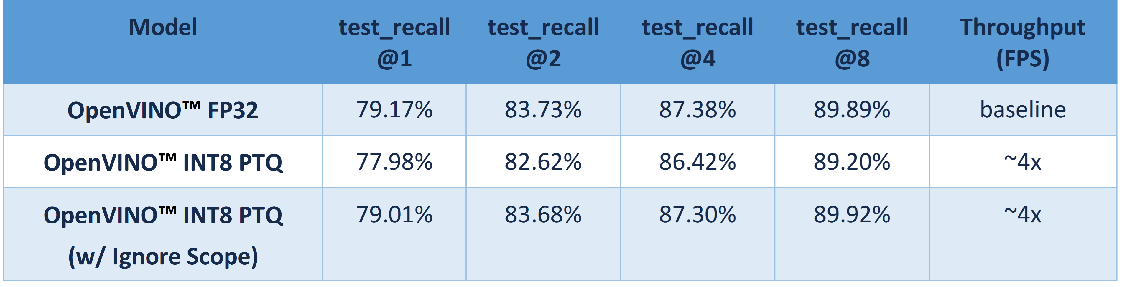
Table 1 shows CGD OpenVINO™ FP32 and INT8 accuracy verification and performance evaluation results with OpenVINO™ 2023.0 on Intel® Xeon® Platinum 8358 Processor.
From an accuracy perspective, test_recall@1/2/4/8 measures if the top n image retrieval results match with the query image. OpenVINO™ INT8 PTQ quantizes all FP32 layers to INT8, which leads to ~1.2% accuracy degradation compared with OpenVINO™ FP32 Model. OpenVINO™ INT8 PTQ (w/ IgnoreScope) skips quantization of accuracy sensitive layers via ignore scopes, which controls the accuracy difference between OpenVINO™ INT8 model and OpenVINO™FP32 model within 0.16%.
Compared with OpenVINO™ FP32 model, both OpenVINO™ INT8 PTQ and OpenVINO™ INT8 PTQ (w/ Ignore Scopes) can reach ~4x performance boost. Results show that keeping serval layers as FP32 precision has minimal impact on OpenVINO™ INT8 model.
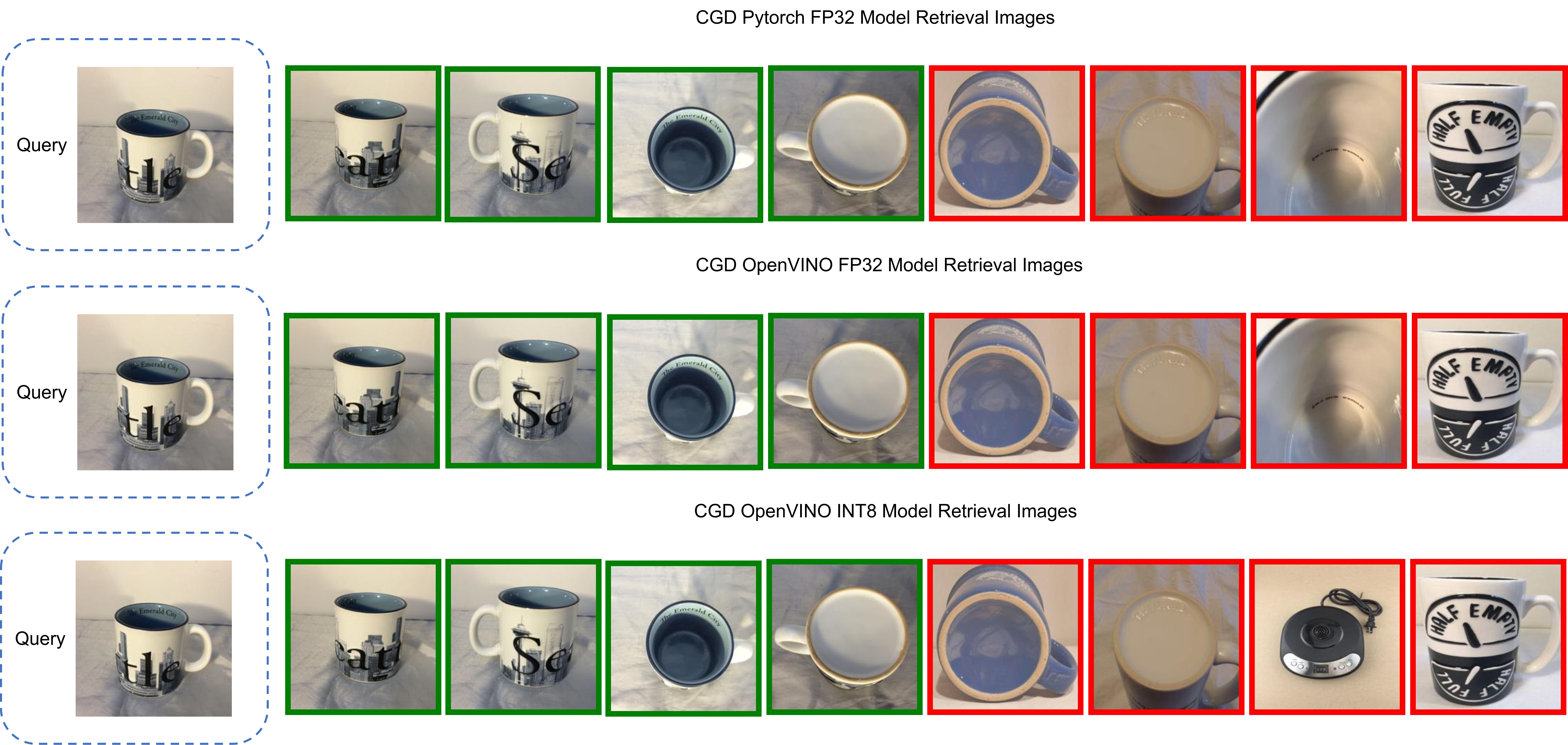
Figure 5 shows the CGD Image Retrieval Results of Pytorch FP32, OpenVINO™ FP32/INT8 models with the same query image. The Pytorch and OpenVINO™ FP32 retrieved images are the same. Although the 7th image of OpenVINO™ INT8 model results is not matched with FP32 model's results, it can be further filtered out with predicted class information.
Conclusion
In this blog, we introduced how to enable and quantize the CGD model with OpenVINO™ runtime and NNCF:
- Proposed INT8 quantization NNCF PTQ with ignore scopes to reach ~4x performance boost while keeping minimal accuracy degradation (<0.16%) compared to FP32 model.
- Provided a demo repository for CGD model enabling, quantization, accuracy verification, and deployment with OpenVINO™ and NNCF.
Reference
OpenVINO™ model transformation –MHA subgraph optimization
Authors:Kunda Xu, Yi Zhang, Chenhu Wang
Introduction
Due to significant advancements in microprocessor technologies, computational ability has grown faster than the memory bandwidth over the past decades. As a result, most linear operations in vector space are memory-bounded, so the execution time is limited by the memory bandwidth. The rare exceptions include convolutions and matrix multiplications. These exceptions could be especially important for some workloads, so a lot of vectorization and parallelization works are done to increase their computational throughput (Advanced Matrix Registers for example). In this blog, let’s focus on the optimization methods on low parallel efficiency and memory-bounded operations which are widely used in transformers models. And we will introduce how to use OpenVINO™ transformations feature and will use a sample with MHA fusion optimization to show.
In this blog, we will introduce optimization technics of OpenVINO™ for model structure from the following angles.
- MHA subgraph structure and optimization method.
- OpenVINO™ model transformation introduction- new feature Snippets
- Case study: MHA subgraph OpenVINO optimization
Requirement
OpenVINO >= 2023.0
OpenVINO™ is an open-source toolkit for optimizing and deploying AI inference which can boost deep learning performance in computer vision, automatic speech recognition, natural language processing and other common tasks.
Reference: OpenVINO™ install guide - Linux
MHA structure and optimization method
Multi-Head Attention (MHA) is a key component in the Transformer model used in NLP. It enhances representation and modeling by learning multiple sets of attention weights simultaneously, allowing the model to capture diverse patterns and dependencies. MHA enables parallel computation, improves robustness by filtering out noise, and scales well for longer sequences. Overall, MHA enhances the Transformer model's capabilities and improves performance in various NLP tasks.
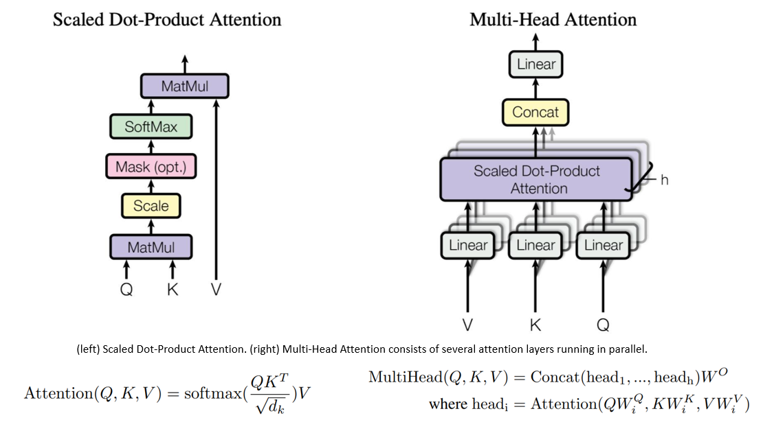
Each "head" of MHA may focus on different parts of the input, thus enabling the model to capture richer and more diverse information. The characteristics of the attention structure that its excellent context-related ability needs to be exchanged for a large amount of computational complexity and memory resources and will be more complicated during the model training process. An inappropriate learning rate may lead to overfitting of the model or difficulty in converging the model loss function.
Transformers are slow and memory-hungry on long sequences since the time and memory complexity of self-attention are quadratic in sequence length. Approximate attention methods have attempted to address this problem by trading off model quality to reduce the computing complexity.
For the mainly optimized workflow, there are two main optimization points:
- MHA calculation logic optimization, optimize the utilization rate of CPU cache in the model calculation process, reduce the time overhead of data copy, improve the utilization rate of data in the cache and improve the performance of hot point operator attention.
- MHA operator fusion optimization, through the operation of operator fusion and subgraph fusion, the IO cost of data will be reduced, and the inference performance of the model will be improved.
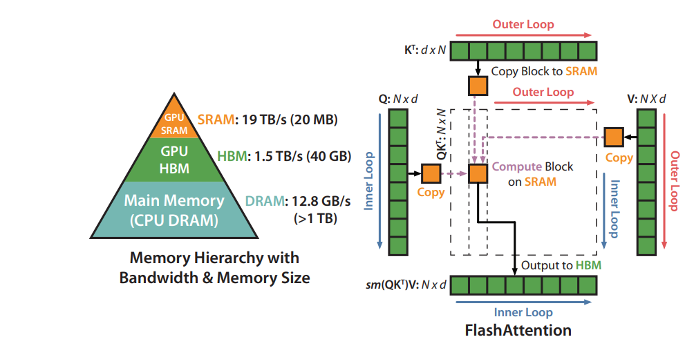
Based on above two optimization points, we found a mature solution called “FlashAttention” which already been proposed for discrete GPU(dGPU) computing optimization. So that we reference FlashAttention, a new attention algorithm that computes exact attention with far fewer memory accesses, to optimize the attention subgraph on CPU.
FlashAttention subgraph optimization workflow
The original FlashAttention algorithm on dGPU uses tiling to prevent materialization of the large 𝑁 × 𝑁 attention matrix (dotted box) on (relatively) slow GPU HBM. In the outer loop (red arrows), FlashAttention loops through blocks of the K and V matrices and loads them to fast on-chip SRAM. In each block, FlashAttention loops over blocks of Q matrix (blue arrows), loading them to SRAM, and writing the output of the attention computation back to HBM.
Using OpenVINO transformation feature instruction, we optimize the data flow about MHA subgraph, Since the algorithm is planned to use on the CPU, we need to optimize the memory usage and calculation process between the caches at each level of the CPU. And the optimized data workflow about MHA subgraph which integrated in the OpenVINO, the graph is shown like below.
OpenVINO MHA subgraph optimization workflow
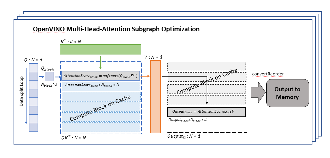
We divide the Q matrix into Q_block (shape is N_block*d) in the dimension of N (sequence tokens length), because the calculation characteristics of SoftMax can support us to calculate the data of each row separately, so that we can ensure that the K matrix is consistent with each During the calculation of Q_block, the data of the K matrix can be stored in the CPU cache, reducing the time overhead caused by data transfer in memory and cache, and processing the data of one block at a time can make full use of the computing resources of each core.
An other point to note is that to ensure that the data of each set of K*Q_block can be in the same cache, we need to manually specify that each set of calculations is completed in one thread (OneDNN creates multiple threads for single block computing which the cache cannot be reused, and lead to a worse performance in memory-bound scenarios. It is the main reason do not adopt OneDNN for transformers).
After getting AttentionSorce_block, it can be directly calculated with V matrix, because the size of AttentionSorce_block is N_block*N, the size of the V matrix is N*d, so there is no need to wait until all AttentionSorce calculations completed, and Output_block can be directly calculated, which can reduce the waiting time for data synchronization and further improve calculation efficiency.
After waiting for the calculation of all divided block data to be completed, all the results are spliced, and reorder the output data structure to meet the following node input shape request, and then the data will be copied to the memory.
During the entire MHA subgraph calculation process, by balancing the relationship between the amount of data and the size of the CPU cache, the utilization rate of data in the cache is improved, the time overhead of data transfer is reduced, the utilization rate of advanced caches is fully utilized, the calculation time is reduced, and the performance for computational performance of the operator.
If you want to know more detail about the MHA subgraph optimization implementation, reference MHA node source code.
Reference : MHA node source code
OpenVINO transformations optimization
In OpenVINO's optimization process for the model structure, we can organize it into a pipeline as shown in the figure below. The whole process includes two parts: the structural transformation of nGraph and the transformation of internal plugin graph.
During the nGraph transformation process, modules including common transformations and LPT (Low Precision Transformations) Snippets Tokenizer, etc. will perform some rule-based or automatic compilation structure replacement and optimization on the graph of the model
In the process of internal plugin graph transformation, the optimized nGraph will be deeply optimized for the platform through the optimizer and generator and compiled into kernel execute code that can run on the target platform
In this blog, we will focus on the characteristics and usage of Snippets.
Snippets Architecture
Snippets is known as a graph compiler, a highly specialized compiler for computational graphs.
.png)
Below graph is the detail workflow of Snippets
.png)
Snippets take nGraph model as an input, instead of a source code, the workflow consists of three major blocks: Tokenizer, Optimizer and Generator:
- Tokenizer (the Snippets Frontend) optimize nGraph model and tries to convert to an nGraph IR and stores inside a Subgraph node.
- Optimizer (the Snippets body), to improve the program in a desired way without modification of its meaning.
- Generator (the Snippets Backend) uses the optimized IR to produce executable code.
Snippets Tokenizer algorithm
Tokenizer run on an nGraph model and the main purpose is to identify subgraphs that are suitable for code generation.
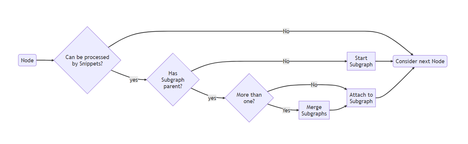
Pattern matching can indeed process only a limited set of predefined operations' configurations, so the relations between the operations are fixed in this case. Thus, the tokenizer's flexibility becomes a significant advantage when the number of new ML topologies increase srapidly, so it becomes more and more expensive to support and extend a large set of patterns.
Snippets Optimizer algorithm
Optimizer consists of three subunits and two are major units: one is performing data flow optimization, and one is focused on control flow,
Data flow optimizer
- Inserts utility operations to make the dataflow explicit and suitable for further optimizations and code generation.
- Replaces some Ops to allow for generation of amore efficient code
IR converts
- Convert from data-flow-oriented representation(nGraph IR) to control-flow-focused IR (Linear IR).
Control flow optimizer
- Common pipeline, auto matic loop injection and loop optimizations
- Buffer pipeline, managing buffer identify and allocate
- Final pipeline, connect Generator modules and release redundant resources.
Case study: MHA subgraph OpenVINO optimization
In this chapter, we take the Bert model as the object of explanation, automatically download and convert the model through the open model zoo, use the Netron tool to view the topology of the model, use the benchmark_app to test the model and save the exec graph of the model, or manually The way to adjust the parameter is to turn on and off the optimization to compare the impact of the MHA operator optimization on the OpenVINO IR model.
First of all, you need to make sure that openvino and openvino-dev packages have been installed. I won’t go into details here. If you don’t know how to install the environment, you can refer to the previous blog content.
Step 1. Models prepare and model convert
Open Model Zoo is a useful toolkit which include model downloader, model converter, model quantization etc. to easily enable model by OpenVINO™,
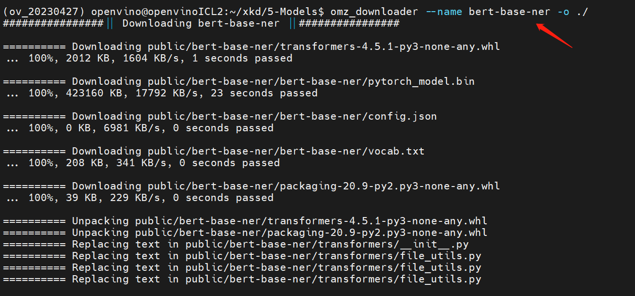
Using following commend-line (cmd) to download “bert-base-ner” original model by omz_downloader
bert-base-ner is a fine-tuned BERT model that is ready to use for Named Entity Recognition and achieves state-of-the-art performance for the NER task.
Using following commend-line (cmd) to auto convert “bert-base-ner” original model to OpenVINO™ IR model by omz_converter
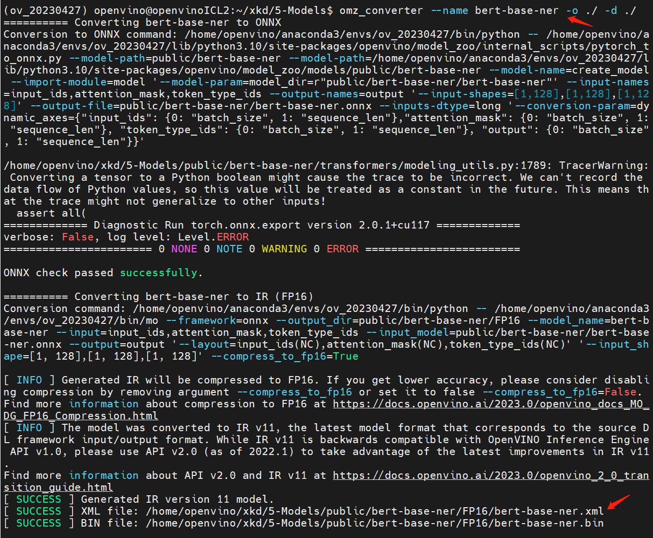
Now, we get the “bert-base-ner” IR model , and we can use benchmark_app to evaluate it on our device.
Step 2. Check model exec-graph
OpenVINO™ benchmark_app is a versatile tool, it can evaluate model’s performance ,analysis model hotspot operate, and also can help us to analysis to model’s topology graph. IR save the topology graph in .xml file, but this graph is not including all optimization graph, so that we can save the execution graph to check the runtime graph on target device.
The exec-graph will save as “bert-base-ner-exec.xml”, and use Netron to check the original IR graph and the execution IR graph
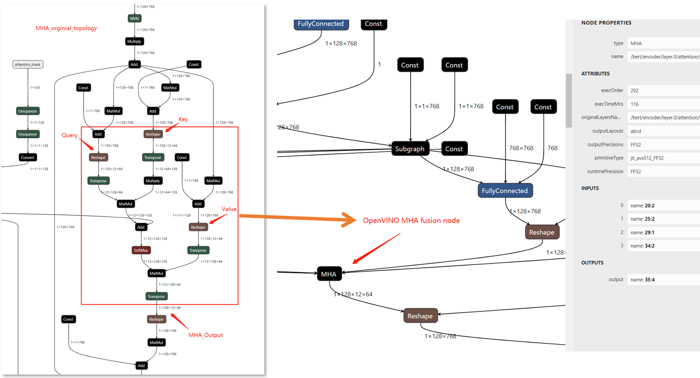
In the compare figure, we can find that the MHA subgraph as been optimize as a fusion graph named MHA, but there is only a single node, If we want to check the fusion node inside we should add some config in OpenVINO to show the detail information about it.
So that, we can simply insert below serialization code
after code line https://github.com/openvinotoolkit/openvino/blob/master/src/plugins/intel_cpu/src/nodes/subgraph.cpp#L81
which will dump all subgraphs topology with it's friendly name in execution graph.
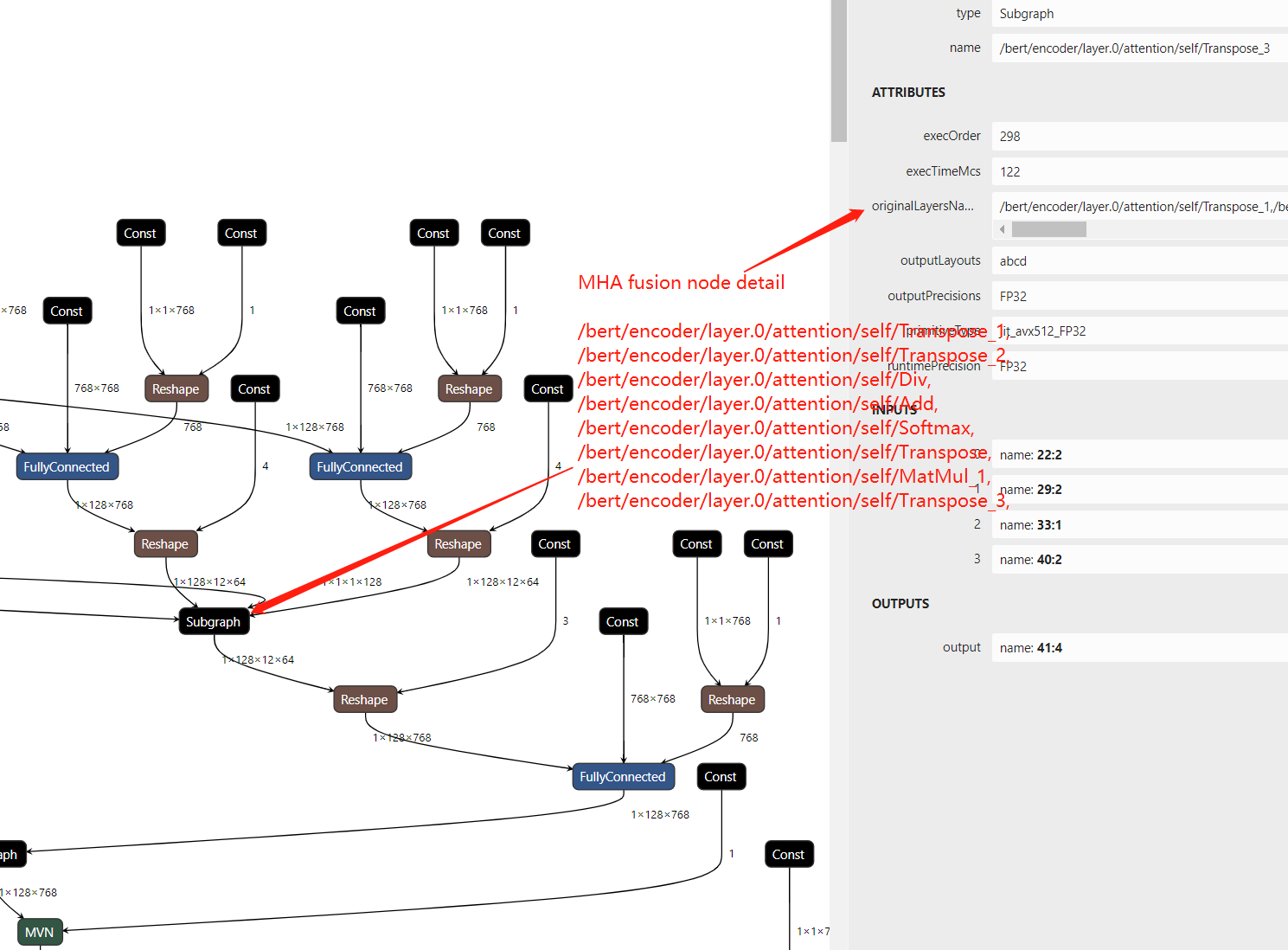
Now, re-build OpenVINO™ from source code and save the execution graph we will find the subgraph include the parameter “originalLayersName” which means that which layers are fusion in MHA subgraph.
Step 3. Close Snippets optimization
Snippets as an automate optimization method which default open at every time. And if you don’t want to use automatic method and replace by any custom algometric, Snippets can be open/close by config in the model compile process, so that we can change the Snippets config key by “KEY_SNIPPETS_MODE” for expected values parameter “ENABLE(default) / DISABLE / IGNORE_CALLBACK”.
In benchmark_app case we should edit a config .json file to save the ov::config
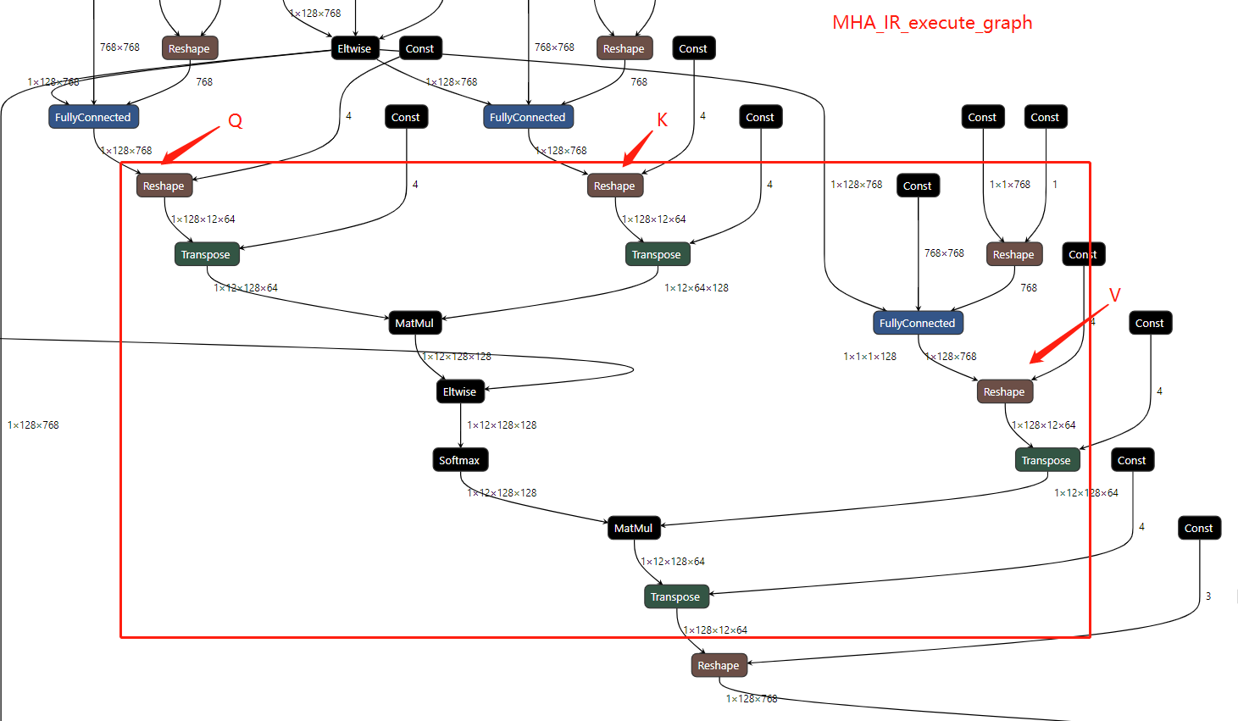
And then use the config file by “-load_config” parameter to run benchmark_app and save a exec-graph, we will find the MHA fusion node is deconstruct.
Now open the new execution graph we can find the transformation optimized MHA fusion node has remove.
Conclusion
In this blog, we show MHA subgraph fusion optimization by OpenVINO™ , highlight to newfeature Snippets in transformations and introduce the MHA fusion node optimization ideas in terms of CPU memory-bounded.
Please note, this optimization idea can be used on likely transformer structure models by OpenVINO™. But whether the above MHA fusion node will be used it need to analysis case-by-case.
We will continue to optimize performance along with upgrading OpenVINO™ for model scaling such as Bert-base , GPT and any others LLM to get latest efficient support with OpenVINO™ backend.
Reference
OpenVINO™ MHA fusion node
OpenVINO™ Snippets Design Guide
[Paper] FlashAttention: Fast and Memory-Efficient Exact Attention with IO-Awareness
[Paper] AttentionIs All You Need
AquilaChat-7B Language Model Enabling with Hugging Face Optimum Intel
Introduction
What is AquilaChat-7B Language Model?

Aquila Language Model is a set of open-source large language models (LLMs) developed by the Beijing Academy of Artificial Intelligence (BAAI). Aquila models support both Chinese and English, commercial license agreements, and compliance with Chinese domestic data regulations.
AquilaChat-7B is a conversational language model that supports Chinese and English dialogue. It is based on the Aquila-7B foundation model and fine-tuned using supervised fine-tuning (SFT). AquilaChat-7B original Pytorch model and configurations are publicly available here.
Hugging Face Optimum Intel

Hugging Face is one of the most popular open-source data science and machine learning platforms. It acts as a hub for AI experts and enthusiasts—like a GitHub for AI. Over 200,000 models are available across Natural language processing, Multimodal models, Computer Vision, and Audio domains.
Hugging Face provides wide support for model optimization and deployment of open-sourced LLMs such as LLaMA, Bloom, GPT-Neox, Dolly 2.0, to name a few. More details please refer to Open LLM Leaderboard.
Optimum-Intel provides a simple interface between the Hugging Face and OpenVINOTM ecosystem to leverage high-performance inference capabilities for Intel architecture. Here is a simple example to show how to run Dolly 2.0 models with OVModelForCausalLM using OpenVINOTM runtime.
Hola! So, for LLMs already supported by Hugging Face transformers and optimum, we can smoothly switch the model inference backend from Pytorch to OpenVINOTM by changing only two lines of code.
However, what if an LLM from an open-source community that not native supported by Hugging Face Transformers library? How can we still leverage the tools of Hugging Face and OpenVINOTM ecosystem for model optimization and deployment?
Indeed, AquilaChat-7B is a custom model for the Hugging Face Transformers. So, we use it as an example to elaborate the custom model enabling methodology step by step.
How to Enable a Custom Model on Hugging Face?
To leverage the Hugging Face ecosystem and optimization for AquilaChat-7B model, we need to convert the original Pytorch model to Hugging Face Format. Before we dive into conversion details, we need to figure out what is AquilaChat-7B’s model structure, tokenizer, and configurations.
According to Aquila’s official model description:
“The Aquila language model inherits the architectural design advantages of GPT-3 and LLaMA, replacing a batch of more efficient underlying operator implementations and redesigning the tokenizer for Chinese-English bilingual support. The Aquila language model is trained from scratch on high-quality Chinese and English corpora. “
Model Structure and Tokenizer
For model structure, Aquila Model adopts the original Meta LLaMA pytorch implementation, which combines RMSNorm (GPT-3) to improve training stability and Rotary Position Embedding (GPT-NeoX)to incorporate explicit relative position dependency in self-attention.
For tokenizer, instead of using byte-pair encoding (BPE) algorithms implemented by Sentence Piece, Aquila re-trained HuggingFace GPT-NeoX tokenizer with extended vocabulary (vocab_size =100008, including 8 special tokens, e.g. bos_token=100006, eos_token=100007, unk=0, pad=0 used for inference based on here.
Rotary Position Embedding
Rotary Position Embedding (RoPE) encodes the absolute position with a rotation matrix and meanwhile incorporates the explicit relative position dependency in the self-attention formulation. Compare to other position embedding methods, RoPE provides valuable properties such as flexibility of sequence length, long-term decay, and linear self-attention with relative position embedding. Based on the original paper, there are two mainstream implementations of RoPE:
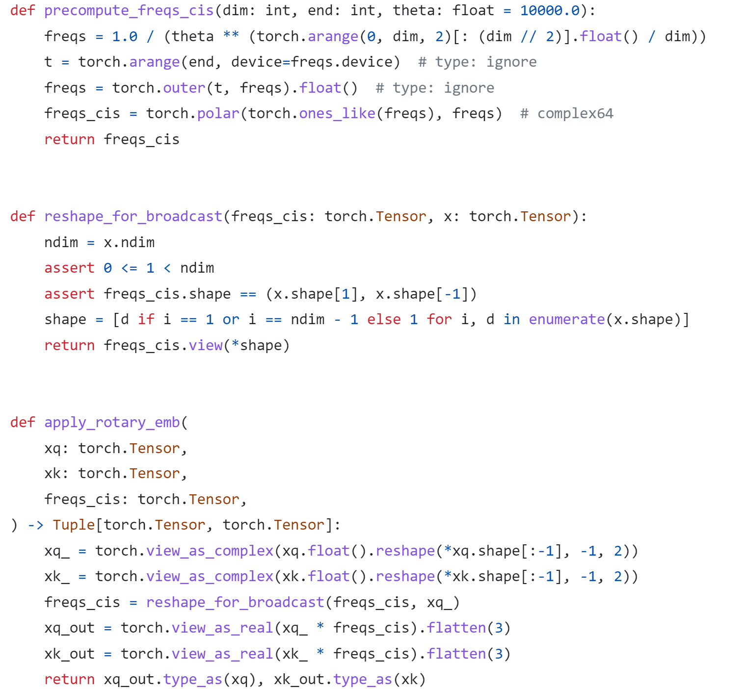
As show in Figure 3, Meta LLaMA’s implementation directly use complex number to calculate rotary position embedding.
As show in Figure 4, Google PaLM’s implementation expands the complex number operation and calculate sinusoidal functions in matrix equation of real numbers.
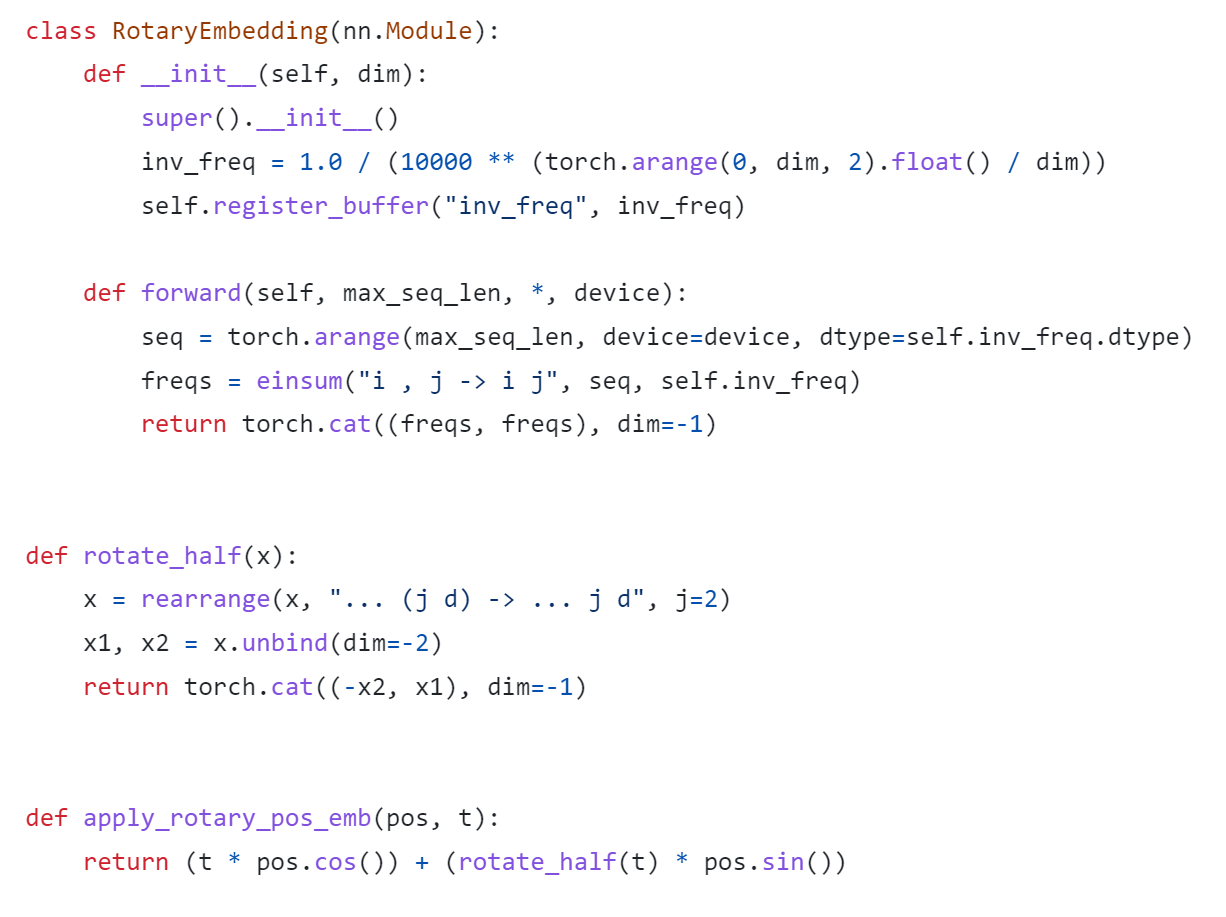
Both RoPE implementations are valid for the Pytorch model. Hugging Face LLaMA implementation adopts PaLM’s RoPE implementation due to the limitation of complex type support for ONNX export.
Besides, Hugging Face provides a useful script convert_llama_weights_to_hf.py to convert the original Meta LLaMA Pytorch Model to Hugging Face Format as follows:
- Extract Pytorch weights and convert Meta LlaMA RoPE implementation to Hugging Face RoPE implementation.
- Convert tokenizer.model trained with Sentence Piece to Hugging Face LLaMA tokenizer.
Convert AquilaChat-7B Model to Hugging Face Format
Similarly, we provide a convert_aquila_weights_to_hf.py to convert AquilaChat-7B Model to Hugging Face Format.
- Extract Pytorch weights and convert Aquila RoPE implementation to Hugging Face RoPE implementation
- Initialize and save a Hugging Face GPT-NeoX Tokenizer with extended vocabulary based on original tokenizer configurations provided by Aquila.
- Add a modeling_aquila.py to enable support forAutoModelForCausalLM and AutoTokenizer
Here is the converted Hugging Face version of AquilaChat-7B v0.6 model uploaded in Hugging Face.
You may convert pytorch weights to Hugging Face format in two steps:
- Download AquilaChat-7B Pytorch Model and configurations here
- Convert AquilaChat-7B Pytorch Model and configurations to Hugging Face Format
Hugging Face AquilaChat-7B Demo
Setup Environment
Run inference with AutoModelForCausalLM
Run inference with OVModelForCausalLM
Conclusion
In this blog, we show how to convert a custom Large Language Model (LLM) to Hugging Face format to leverage efficient optimization and deployment with Hugging Face and OpenVINOTM Ecosystem.
Please note, this is the initial model enabling step for AquilaChat-7B model with OpenVINOTM. We will continue to optimize performance along with upgrading OpenVINOTM for LLM scaling. Please refer to OpenVINOTM and Optimum-Intel official release to get latest efficient support for LLMs with OpenVINOTM backend.
Reference
- FlagAI AquilaChat-7B
- AquilaChat-7B Hugging Face Model
- Hugging Face Optimum Intel
- LLaMA:Open and Efficient Foundation Language Models
- RoFormer:Enhanced Transformer with Rotary Position Embedding
- RotaryEmbeddings: A Relative Revolution
Enable chatGLM by creating OpenVINO™ stateful model and runtime pipeline
Authors: Zhen Zhao(Fiona), Cheng Luo, Tingqian Li, Wenyi Zou
Introduction
Since the Large Language Models (LLMs) become the hot topic, a lot Chinese language models have been developed and actively deployed in optimization platforms. chatGLM is one of the popular Chinese LLMs which are widely been evaluated. However, ChatGLM model is not yet a native model in Transformers, which means there remains support gap in official optimum. In this blog, we provide a quick workaround to re-construct the model structure by OpenVINO™ opset contains custom optimized nodes for chatGLM specifically and these nodes has been highly optimized by AMX intrinsic and MHA fusion.
*Please note, this blog only introduces a workaround of optimization method by creating OpenVINO™ stateful model for chatGLM. This workaround has limitation of platform, which requires to use Intel® 4th Xeon Sapphire Rapids with AMX optimization. We do not promise the maintenance of this workaround.
Source link: https://github.com/luo-cheng2021/openvino/tree/luocheng/chatglm_custom/tools/gpt
To support more LLMs, including llama, chatglm2, gpt-neox/dolly, gpt-j and falcon. You can refer this link which not limited on SPR platform, also can compute from Core to Xeon:
Source link: https://github.com/luo-cheng2021/ov.cpu.llm.experimental
ChatGLM model brief
If we check with original model source of chatGLM, we can find that the ChatGLM is not compatible with Optimum ModelForCasualML, it defines the new class ChatGLMForConditionalGeneration. This model has 3 main modules (embedding, GLMBlock layers and lm_logits) during the pipeline loop, the structure is like below:
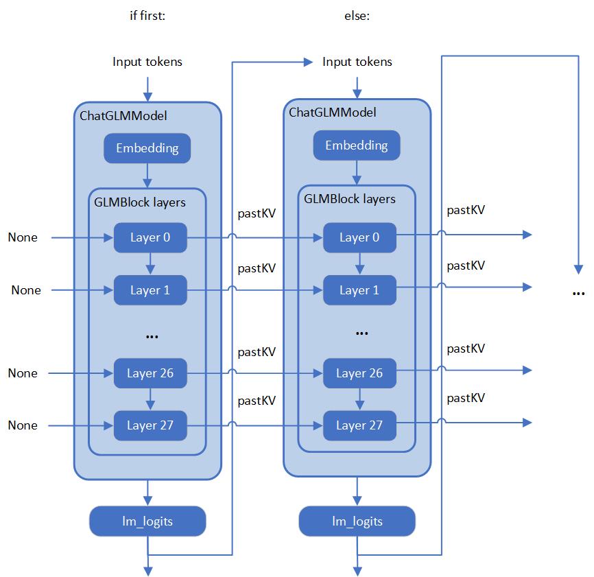
As you can see, the whole pipeline actually require model with two different graphs, the first-time inference with input prompt tokens do not require KV cache as inputs for GLMBlock layers. Since the second iteration, the previous results of QKV Attention should become the inputs of current round model inference. Along with the length of generated token increased, there will remain a lot of large sized memory copies between model inputs and outputs during pipeline inference. We can use ChatGLM6b default model configurations as an example, the memory copies between input and output arrays are like below pseudocode:
Therefore, two topics is the most important:
- How we can optimize model inference pipeline to eliminate memory copy between model inputs and outputs
- How we can put optimization efforts on GLMBlock module by reinvent execution graph
Extremely optimization by OpenVINO™ stateful model
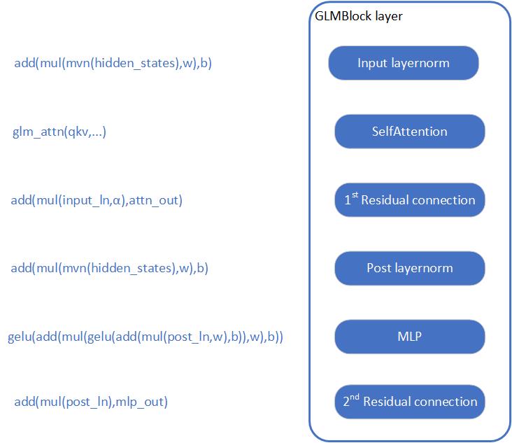
Firstly, we need to analyze the structure of GLMBlock layer, and try to encapsulate a class to invoke OpenVINO™ opset with below workflow. Then serialize the graph to IR model(.xml, .bin).
To build an OpenVINO™ stateful model, you can refer to this document to learn.
https://docs.openvino.ai/2022.3/openvino_docs_OV_UG_network_state_intro.html
OpenVINO™ also provide model creation sample to show how to build a model by opset.
https://github.com/openvinotoolkit/openvino/blob/master/samples/cpp/model_creation_sample/main.cpp
It is clear to show that the emphasized optimization block is the custom op of Attention for chatGLM. The main idea is to build up a global context to store and update pastKV results internally, and then use intrinsic optimization for Rotary Embedding and Multi-Head Attentions. In this blog, we provide an optimized the attention structure of chatGLM with AMX intrinsic operators.
At the same time, we use int8 to compress the weights of the Fully Connected layer, you are not required to compress the model by Post Training Quantization (PTQ) or process with framework for Quantization Aware Training(QAT).
Create OpenVINO™ stateful model for chatGLM
Please prepare your hardware and software environment like below and follow the steps to optimize the chatGLM:
Hardware requirements
Intel® 4th Xeon platform(codename Sapphire Rapids) and above
Software Validation Environment
Ubuntu 22.04.1 LTS
python 3.10.11 for OpenVINO™ Runtime Python API
GCC 11.3.0 to build OpenVINO™ Runtime
cmake 3.26.4
Building OpenVINO™ Source
- Install system dependency and setup environment
- Create and enable python virtual environment
- Install python dependency
- Build OpenVINO™ with GCC 11.3.0
- Clone OpenVINO™ and update submodule
- Install python dependency for building python wheels
- Create build directory
- Build OpenVINO™ with CMake
- Install built python wheel for OpenVINO™ runtime and openvino-dev tools
- Check system gcc version and conda runtime gcc version. If the system gcc version is higher than conda gcc version like below, you should update conda gcc version for OpenVINO runtime. (Optional)
- convert pytorch model to OpenVINO™ IR
Use OpenVINO Runtime API to build Inference pipeline for chatGLM
We provide a demo by using transformers and OpenVINO™ runtime API to build the inference pipeline. In test_chatglm.py, we create a new class which inherit from transformers.PreTrainedModel. And we update the forward function by build up model inference pipeline with OpenVINO™ runtime Python API. Other member functions are migrated from ChatGLMForConditionalGeneration from modeling_chatglm.py, so that, we can make sure the input preparation work, set_random_seed, tokenizer/detokenizer and left pipelined operation can be totally same as original model source.
To enable the int8 weights compress, you just need a simple environment variable USE_INT8_WEIGHT=1. That is because during the model generation, we use int8 to compress the weights of the Fully Connected layer, and then it can use int8 weights to inference on runtime, you are not required to compress the model by framework or quantization tools.
Please follow below steps to test the chatGLM with OpenVINO™ runtime pipeline:
- Run bf16 model
- Run int8 model
Weights compression reduces memory bandwidth utilization to improve inference speed
We use VTune for performance comparison analysis of model weights bf16 and int8. Comparative analysis of memory bandwidth and CPI rate (Table 1). When model weight is compressed to int8, it can reduce memory bandwidth utilization and CPI rate.
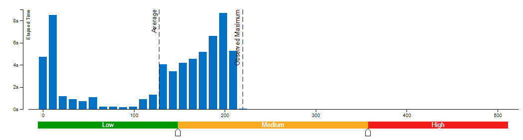
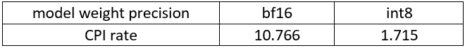
Clockticks per Instructions Retired(CPI) event ratio, also known as Cycles per Instructions, is one of the basic performance metrics for the hardware event-based sampling collection, also known as Performance Monitoring Counter (PMC) analysis in the sampling mode. This ratio is calculated by dividing the number of unhalted processor cycles(Clockticks) by the number of instructions retired. On each processor the exact events used to count clockticks and instructions retired may be different, but VTune Profiler knows the correct ones to use.
A CPI < 1 is typical for instruction bound code, while a CPI > 1 may show up for a stall cycle bound application, also likely memory bound.
Conclusion
Along with the upgrading of OpenVINO™ main branch, the optimization work in this workaround will be generalized and integrated into official release. It will be helpful to scale more LLMs model usage. Please refer OpenVINO™ official release and Optimum-intel OpenVINO™ backend to get official and efficient support for LLMs.
Joint Pruning, Quantization and Distillation for Efficient Inference of Transformers
Introduction
Pre-trained transformer models are widely deployed for various NLP tasks such as text classification, question answering, and generation task. The recent trend is that models continue to scale while yielding improved performance. However, growth of transformers also leads to great amount of compute resources and energy needed for deployment. The goal of model compression is to achieve model simplification from the original without significantly diminished accuracy. Pruning, quantization, and knowledge distillation are the three most popular model compression techniques for deep learning models. Pruning is a technique for reducing the size of a model to improve efficiency or performance. By reducing the number of bits needed to represent data, quantization can significantly reduce storage and computational requirements. Knowledge distillation involves training a small model to imitate the behavior of a larger model.
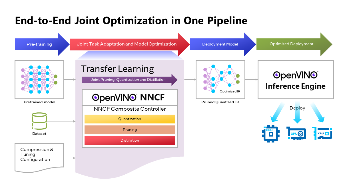
OpenVINOTM Neural Network Compression Framework (NNCF) develops Joint Pruning, Quantization and Distillation (JPQD) as a single joint-optimization pipeline to improve transformer inference performance by pruning, quantization, and distillation in parallel during transfer learning of a pretrained transformer. JPQD alleviates the developer complexity of sequential optimization of different compression techniques, resulting in an optimized model with significant efficiency improvement while preserving good task accuracy. The output of JPQD is a structurally pruned, quantized model in OpenVINOTM IR, which is ready to deploy with OpenVINOTM runtimes optimized on Intel platforms. Optimum intel provides simple API to integrate JPQD into training pipeline for Hugging Face Transformers.
JPQD of BERT-base Model with Optimum Intel
In this blog, we introduce how to apply JPQD to BERT-base model on GLUE benchmark for SST-2 text classification task.
Here is a compression config example with the format that follows NNCF specifications. We specify pruning and quantization in a list of compression algorithms with hyperparameters. The pruning method closely resembles the work of Movement Pruning (Sanh et al., 2020) and Block Pruning For Faster Transformers (Lagunas et al., 2021) for unstructured and structured movement sparsity. Quantization refers to Quantization-aware Training (QAT), see details for QAT in previous blog. At the beginning of training, the model under optimization will be initialized with pruning and quantization operators with this configuration.
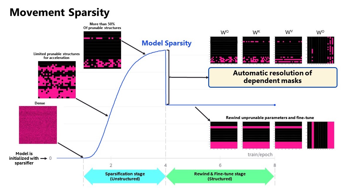
Figure 2 shows the sparsity level of BERT-base model over the optimization lifecycle, including two major stages:
- Unstructured sparsification: In the first stage, model weights are gradually sparsified in the grain size specified by "sparse_structure_by_scopes". The BertAttention layers (Multi-Head Attention: MHA) will be sparsified in 32x32 block size, while BertIntermediate, and BertOutput layers (Feed-Forward Network: FFN) will be sparsified in its row or column respectively. The first stage serves as a warmup stage defined by parameter “warmup_start_epoch” and “warmup_end_epoch”. The “importance_regularization_factor” defines regularization factor onweight importance scores. The factor stays zero before warmup stage, and gradually increases during warmup, finally stays at the fixed value after warmup, users might need some heuristics to find a satisfactory trade-off between sparsity and task accuracy.
- Structured masking and fine-tuning: The first warm-up stage will produce the unstructured sparsified model. Currently, unstructured sparsity optimized inference is only supported on 4th Gen Intel® Xeon® Scalable Processors with OpenVINO 2022.3 or a later version, for details, please refer to Accelerate Inference of Sparse Transformer Models with OpenVINO™ and 4th Gen Intel® Xeon®Scalable Processors. But it is possible to discard some sparse structure entirely from the model to save compute and memory footprint. NNCF provides a mechanism to achieve structured masking by “enable_structured_masking”: true, where it automatically resolves the structured masking between dependent layers and rewinds the sparsified parameters that do not participate in acceleration for task modeling. As Figure 2 shows, the sparsity level has dropped after “warmup_end_epoch” due to structured masking and the model will continue to be fine-tuned.
Known limitation: currently structured pruning with movement sparsity only supports BERT, Wav2vec2, and Swin family of models. See here for more information.
For distillation, the teacher model can be loaded with transformer API, e.g., a BERT-large pre-trained model from Hugging Face Hub. OVTrainingArguments extends transformers’ TrainingArguments with distillation hyperparameters, i.e., distillation weight and temperature for ease of use. The snippet below shows how we load a teacher model and create training arguments with OVTrainingArguments. Subsequently, the teacher model, with the instantiated OVConfig and OVTrainingArguments is fed to OVTrainer. The rest of the pipeline is identical to the native transformers' training, while internally the training is applied with pruning, quantization, and distillation.
Besides, NNCF provides JPQD examples of othertasks, e.g., question answering. Please refer to the examples provided here.
End-to-End JPQD of BERT-base Demo
Set up Python environment with necessary dependencies.
Run text classification example with JPQD of BERT on GLUE
All JPQD configurations and results are saved in ./jpqd-bert-base-ft-$TASK_NAME directory. Optimized OpenVINOTM IR is generated for efficient inference on intel platforms.
BERT-base Performance Evaluation and Accuracy Verification on Xeon
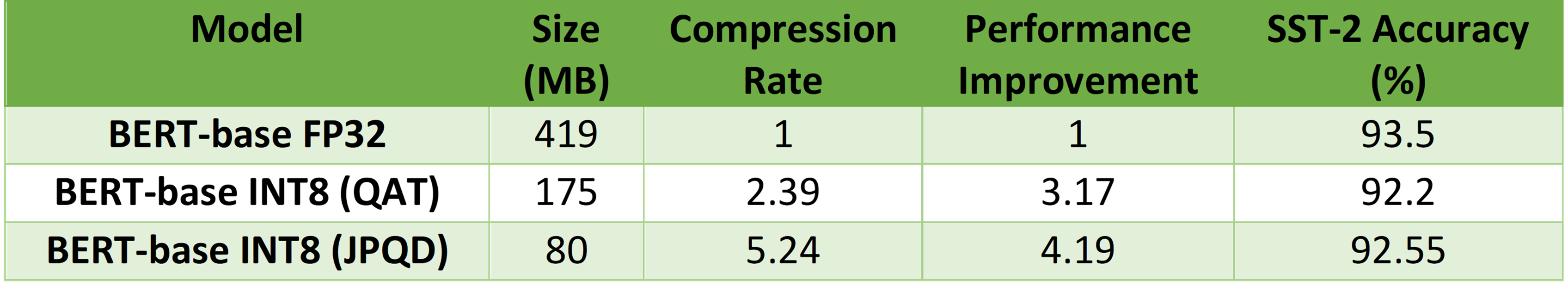
Table 1 shows BERT-base model for text classification task performance evaluation and accuracy verification results on 4th Gen Intel® Xeon® Scalable Processors. BERT-base FP32 model serves as the baseline. BERT-base INT8 (QAT) refers to the model optimized with the 8-bit quantization method only. BERT-base INT8 (JPQD) refers to the model optimized by pruning, quantization, and distillation method.
Here we use benchmark app with performance hint “throughput” to evaluate model performance with input sequence length=128.
As results shows, BERT-base INT8 (QAT) can already reach a 2.39x compression rate and 3.17x performance gain without significant accuracy drop (1.3%) on SST-2 compared with baseline. BERT-base INT8 (JPQD) can further increase compression rate to 5.24x to reach 4.19x performance improvement while keeping minimal accuracy drop (<1%) on SST-2 compared with baseline.
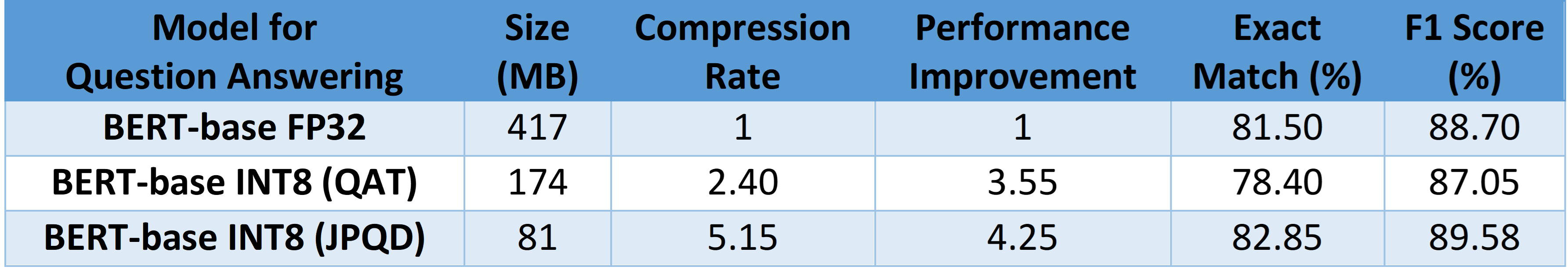
With proper fine-tuning, JPQD can even improve model accuracy while increasing performance in the meantime. Table 2 shows BERT-base model for question answering task performance evaluation and accuracy verification results on 4th Gen Intel® Xeon® Scalable Processors. BERT-base INT8 (JPQD) can increase compression rate to 5.15x to reach 4.25x performance improvement while improving Exact Match (1.35%) and F1 score (1.15%) metric on SQuAD compared with FP32 baseline.
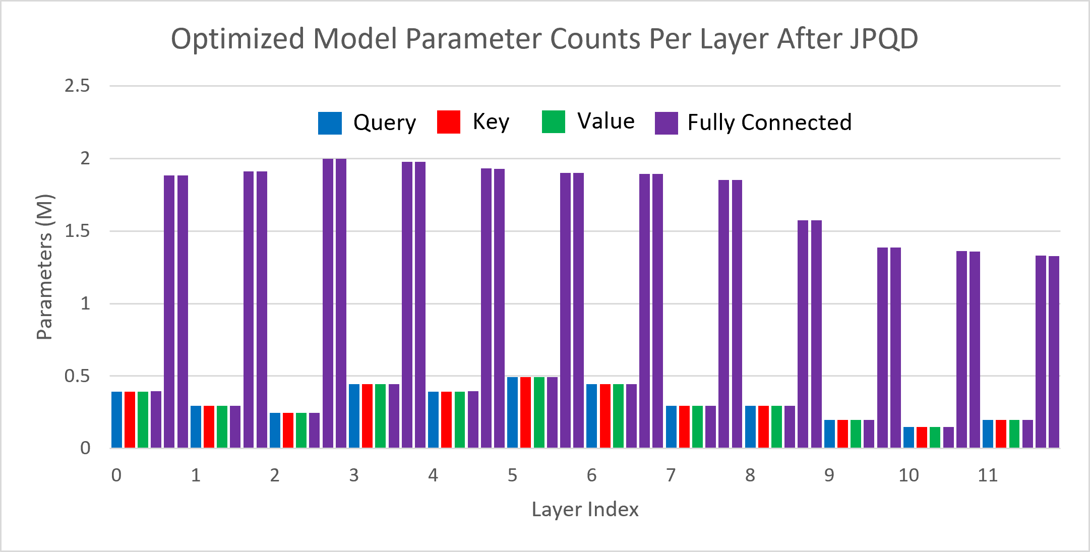
Figure 3 shows the visualization of parameter counts per layer in the BERT-base model optimized by JPQD for the text classification task. You can find that fully connected layers are actually “dense”, while most (Multi-Head Attention) MHA layers will be much sparser compared to the original model.
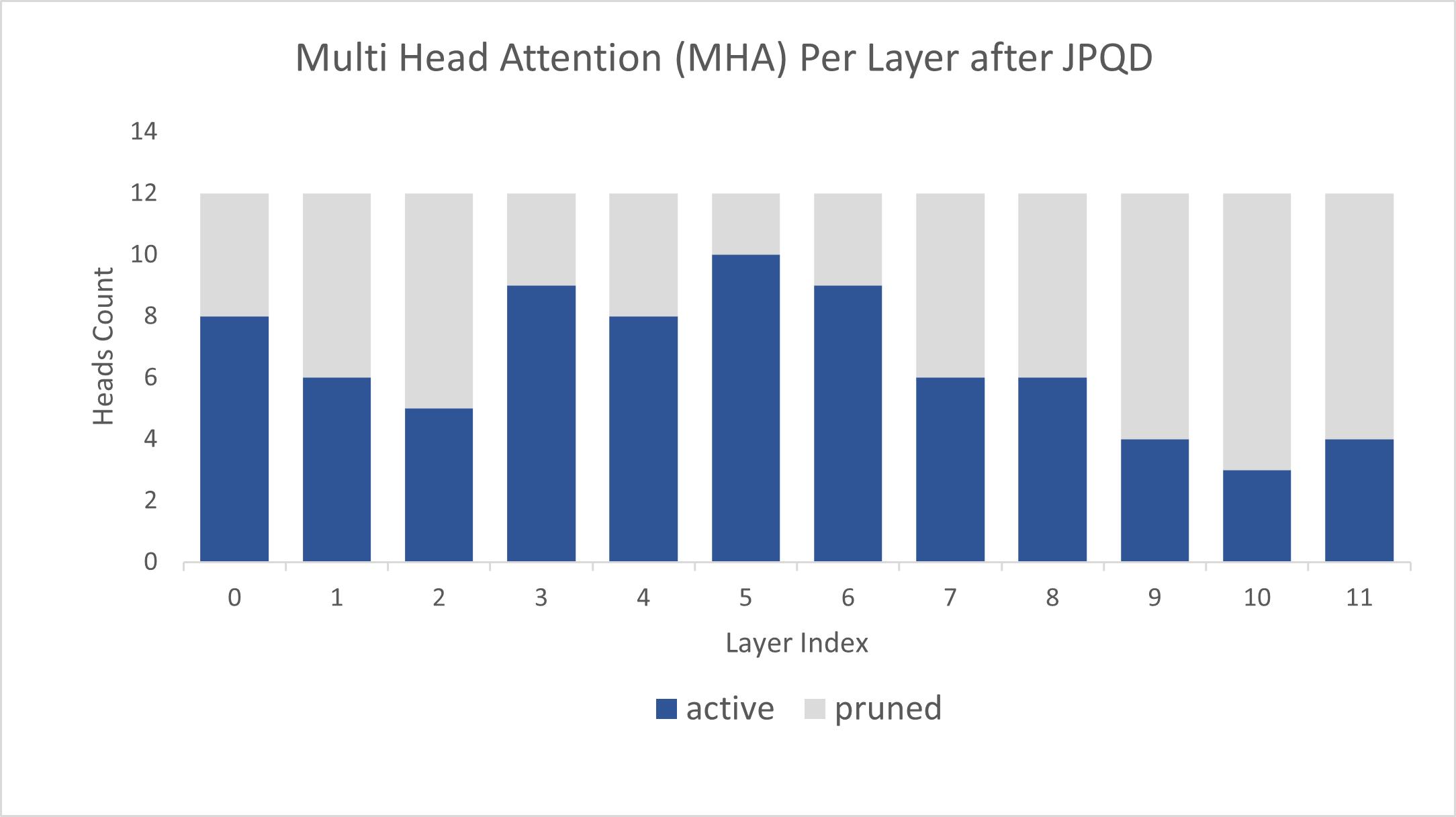
Figure 4 shows MHA head counts per layer in the BERT-base model optimized by JPQD for the text classification task, where active (blue) refer to remaining MHA head counts, while pruned (grey) refers to removed MHA head counts. Instead of pruning uniformly across all MHA heads in transformer layers, we observed that JPQD tends to preserve the weight to the lower layers while heavily pruning the highest layers, similar to experimental results from Movement Pruning (Sanh et al., 2020).
Conclusion
In this blog, we introduce a Joint Pruning, Quantization, and Distillation (JPQD) method to accelerate transformers inference on intel platforms. Here are three key takeaways:
- Optimum Intel provides simple API to integrate JPQD into training pipeline to enable pruning, quantization, and distillation in parallel during transfer learning of a pre-trained transformer. Optimized OpenVINOTM IR will be generated for efficient inference on intel architecture.
- BERT-base INT8 (JPQD) model for text classification task can reach 5.24x compression rate, leading to 4.19x performance improvement on 4th Gen Intel® Xeon® Scalable Processors while keeping minimal accuracy drop (<1%) on SST-2 compared with BERT-base FP32 models.
- BERT-base INT8 (JPQD) model for question answering task can reach 5.15x compression rate to achieve 4.25x performance improvement on 4th Gen Intel® Xeon® Scalable Processors while improving Exact Match (1.35%) and F1 score (1.15%) metric on SQuAD compared with BERT-base FP32 model.
Reference
- Hugging Face Optimum Intel
- Hugging Face Neural Networks Block Movement Pruning
- Intel®Xeon® Processors Are Still the Only CPU With MLPerf Results, Raising the Bar By5x
Additional Resources
Provide Feedback & Report Issues
Notices & Disclaimers
Intel technologies may require enabled hardware, software, or service activation.
No product or component can be absolutely secure.
Your costs and results may vary.
Intel does not control or audit third-party data. You should consult other sources to evaluate accuracy.
Intel disclaims all express and implied warranties, including without limitation, the implied warranties of merchantability, fitness for a particular purpose, and non-infringement, as well as any warranty arising from course of performance, course of dealing, or usage in trade.
No license (express or implied, by estoppel or otherwise) to any intellectual property rights is granted by this document.
© Intel Corporation. Intel, the Intel logo, and other Intel marks are trademarks of Intel Corporation or its subsidiaries. Other names and brands may be claimed as the property of others.